
5.4 Generalisations
5.4.1 Variable end points
So far we have considered
where the value of and were fixed. What happens if we allow the value at the endpoints to vary as well?
5.4.2 One endpoint free
Let’s look at the simplest case: we once again want to find a function such that
| (5.9) |
where , , are fixed but we allow to vary.
In the integration by parts we can now no longer show that the boundary terms are zero, so we need to work through the algebra again to see what happens. As before we make the substitution and expand to first order in with , but without a boundary condition for . Using the techniques employed before, we find
where we have applied the boundary condition in the last line. From the integral we still get the the Euler-Lagrange equation,
but from the boundary term we get an additional equation,
| (5.10) |
Example 5.5:
-
What is the shortest time for a particle to slide along a frictionless wire under the influence of gravity from to for arbitrary ? (A variation on the brachistochrone.)
Solution:
-
From the brachistochrone problem we know that for
and that the Euler-Lagrange equation has the first integral
The solution is still a cycloid,
which indeed passes through for . Now for an extremum of the travel time, we have the additional condition
We conclude , i.e., the cycloid is horizontal at . This occurs when
i.e., when . In that case we can find from
and thus . Finally, .
5.4.3 More than one function: Hamilton’s principle
We often encounter functionals of several functions of the form
| (5.11) |
We now look for stationary points with respect to all , again keeping the functions at the endpoints fixed. Generalising the usual technique for partial derivatives to functional ones, i.e., varying each function in turn keeping all others fixed, we find
The usual integration-by-parts technique thus leads to Euler-Lagrange equations,
| (5.12) |
Hamilton’s principle of least action
An important application in classical dynamics is Hamilton’s principle. Suppose we have a dynamical system defined by “generalised coordinates” , , which fix all spacial positions of a mechanical system at time .
In standard Newtonian mechanics, where the energy is made up of a kinetic energy and potential energy , we can now define an object called the Lagrangian by
| (5.13) |
Example 5.6:
-
Derive Newton’s equation of motion for a particle of mass attached to a spring from the Lagrangian.
Solution:
-
From ( 5.13 ) we find that
or
One interesting consequence of our previous discussion of first integrals, is that they carry over to this problem, and will give us conservation laws.
First of all, let us look what happens if we are looking at an isolated self-interacting system. This means there are no external forces, and thus there can be no explicit time dependence of the Lagrangian,
From experience we expect the total energy to be conserved. Can we verify that?
We know from the case of a functional of a single function,
that the first integral is
The obvious generalisation for this case is
Secondly, what happens if a coordinate is missing from ? In that case we get the first integral
If we identify as the “canonical momentum” , we find that is a constant of motion, i.e., doesn’t change.
The form of mechanics based on Lagrangians is more amenable to generalisation than the use of the Hamiltonian, but it is not as easy to turn it into quantum mechanics. To show its power let us look at a relativistic charge in fixed external E.M. fields, where the Lagrangian takes the (at first sight surprising) form
The first term can be understood by Taylor expansion for small velocities, where we must find , which is the right mixture of a potential ( ) and kinetic term.
The equations of motion take the form (remembering that and depend on )
With a standard definition of and , we have
5.4.4 More dimensions: field equations
For dynamics in more dimensions , we should look at the generalisation of the action,
| (5.14) |
where is an infinitesimal volume in -dimensional space and
| (5.15) |
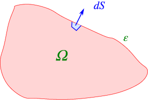
As usual, we now look for a minimum of the action. We make the change , keeping the variations small, but zero on the surface of the region (mathematically, that is sometimes written as ), see Fig. 5.5 .
Looking for variations to first order in , we get
( ). The surface integral vanishes due to the boundary conditions, and requiring , we find the Euler-Lagrange equation,
| (5.16) |
or, more explicitly:
| (5.17) |
The slightly abstract form discussed above can be illustrated for the case of a 1D continuum field (e.g., a displacement), which depends on both position and time . With for and for the E-L equations become
with
For that case the action takes the form
Clearly this suggest that plays the role of Lagrangian, and we call the Lagrange density.
Example 5.7:
-
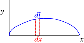
Describe the motion of an elastic stretched string, with fixed endpoints, assuming small deformation, see Fig. 5.6 .
Solution:
-
As per usual, we parametrise the position by , and assume to be small. In that case we have
The mass density of the string remains almost constant, and we find that the contribution to the kinetic energy between and is
The potential energy in that part of the string is the tension times the stretching,
We conclude
and
Using the previous results with , we get
We thus get the wave equation
with .
Example 5.8:
-
Find the equations of motion for a freely moving elastic band of length . For simplicity, assume a two-dimensional world, small stretching, and uniform density.
Discuss the solution to the equations of motion for an almost circular band.
Solution:
-
Specify the points on the band as , with periodic boundary conditions , . The local length is . This needs to be compared to the unstretched band, where (but the band does not have to be circular!). For small stretching, the energy for compression or stretching must be given by a form Hook’s law, i.e, be proportional to the local stretching or compression squared,
At the same time the kinetic energy is given by
Thus,
The EoM are found form a combination of Hamilton’s principle and the field problems discussed above,
If the band is almost circular, we write , and expand to first order in and ,
This can be rewritten as
This shows the conservation law .
Thus, it is easy to solve the case when is independent of and . Then
which describes simple harmonic motion.
Example 5.9:
-
Show that the Lagrangian density (in 3+1 dimensions)
leads to the Klein-Gordon equation.
Solution:
-
First note that the first term is the kinetic energy density, so the next two terms can be interpreted as minus the potential energy. There is some amiguity to this, since we have
the action for a relativistic(covariant) field theory.
From the Euler-Lagrange equations we find that
leading to the Klein-Gordon equation, a slightly modified form of the wave-equation, describing a field with modes with mass –i.e., a classical description of massive bosons.
5.4.5 Higher derivatives
Occasionally we encounter problems where the functional contains higher than first order derivatives; much what we have said above is of course rather specific to the case of first order derivatives only!
This work is a UK OER project as part of the Skills for Scientists project. Please contact Niels Walet for more information
 This work is licensed under a Creative Commons Attribution-Noncommercial-Share Alike 2.0 Generic License