
2.3 Polar Coordinates
L&T, 1.9.3.3
The position of any point in two-dimensional space can be specified by giving its coordinates. However we could also say where is by giving the distance from the origin , and the direction we need to go.
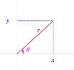
These two quantities are the polar coordinates of P. From a right angled triangle we see that , and , so , and thus . (N.B. We always take positive square root here!) Also , Therefore . In this case we must always draw a diagram. The reason is that two different angles can have the same tangent. The only relevant once for polar coordinates are that , when . If is in first or second quadrant we use , and if is in third or fourth quadrant we use . So always draw a little sketch!
Example 2.10:
-
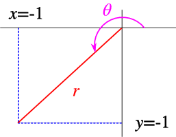
Find the polar coordinates corresponding to .
Solution:
-
, and . From the sketch we see that
2.3.1 Polar curves
Often we wish to draw curves in polar coordinates; the most important example are the Kepler orbits, the ones resulting from a particle moving in the gravitational fiels of a single orbit, e.g., a single planet/comet orbiting the sun.
The Kepler orbits can be shown to take the form
Here is a quantity with unit length, determined from masses and gravitational parameters. We now use this relation (with , for simplicity) to find the typical orbits for , (we shall choose ), , and (we shall choose 2).
In order to plot these results we rewrite the relation as
and plot the value of for each (or a suitably chosen selection).
This is a circle.
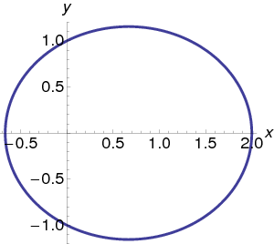
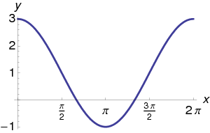
In this case it is not very hard to solve the problem: All values of give a positive , and the easiest solution is just to plot a suitable large number of values. Obvious choices are , and these immediately lead to the elliptical structure shown in Fig. 2.11 . It can be shown that this is a real ellipse, with the origin (the sun around which the palnet revolves) as one of the focusses of the ellipse.
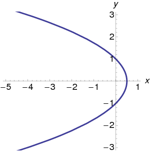
In this case we cannot use , and we thus conclude that the curve moves away to infinity. Once again we can draw a large number of points and we find a parabola, see Fig. 2.12 .
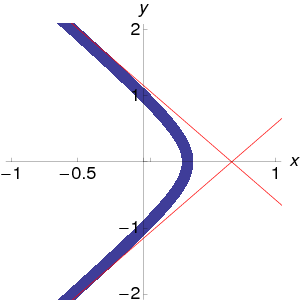
We need to carefully find the allowed range for , see Fig. 2.13 , and we conclude that . Near the end points diverges, and we can actually expand the value of in the behaviour near these two points (Callenge question: how?) to find the two asymptotes , which as we can see from Fig. 2.14 are indeed correct. The curve obtained is a hyperbola.
This work is a UK OER project as part of the Skills for Scientists project. Please contact Niels Walet for more information
 This work is licensed under a Creative Commons Attribution-Noncommercial-Share Alike 2.0 Generic License