
6.2 New variables
In order to understand the solution in all mathematical details we make a change of variables
| (6.2) |
We write . We find
We thus conclude that
| (6.4) |
An equation of the type can easily be solved by subsequent integration with respect to and . First solve for the dependence,
| (6.5) |
where is any function of only. Now solve this equation for the dependence,
| (6.6) |
In other words,
with and arbitrary functions.
6.2.1 Infinite String
This equation is quite useful in practical applications. Let us first look at how to use this when we have an infinite system (no limits on ). Assume that we are treating a problem with initial conditions
| (6.7) |
Let me assume . I shall assume this also holds for and (we don’t have to, but this removes some arbitrary constants that don’t play a rôle in ). We find
The last equation can be massaged a bit to give
| (6.9) |
Note that is the integral over . So will always be a continuous function, even if is not!
And in the end we have
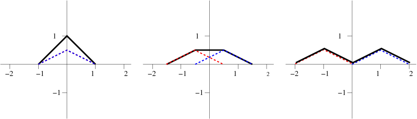
Suppose we choose (for simplicity we take )
| (6.11) |
and . The solution is then simply given by
| (6.12) |
This can easily be solved graphically, as shown in Fig. 6.2 .
6.2.2 Finite String
The case of a finite string is more complex. There we encounter the problem that even though and are only known for , can take any value from to . So we have to figure out a way to continue the function beyond the length of the string. The way to do that depends on the kind of boundary conditions: Here we shall only consider a string fixed at its ends.
Initially we can follow the approach for the infinite string as sketched above, and we find that
Look at the boundary condition . It shows that
| (6.15) |
Now we understand that and are completely arbitrary functions – we can pick any form for the initial conditions we want. Thus the relation found above can only hold when both terms are zero
Now apply the other boundary condition, and find
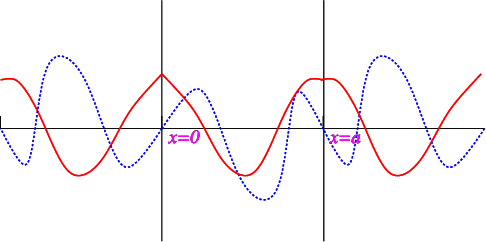
The reflection conditions for and are similar to those for sines and cosines, and as we can see from Fig. 6.3 both and have period .
This work is a UK OER project as part of the Skills for Scientists project. Please contact Niels Walet for more information
 This work is licensed under a Creative Commons Attribution-Noncommercial-Share Alike 2.0 Generic License