
11.1 Modelling the eye
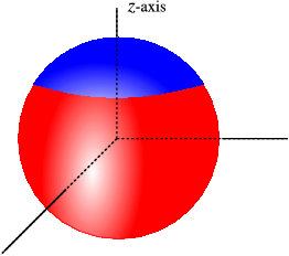
Let me model the temperature in a simple model of the eye, where the eye is a sphere, and the eyelids are circular. In that case we can put the -axis straight through the middle of the eye, and we can assume that the temperature does only depend on and not on . We assume that the part of the eye in contact with air is at a temperature of C, and the part in contact with the body is at C. If we look for the steady state temperature it is described by Laplace’s equation,
| (11.1) |
Expressing the Laplacian in spherical coordinates (see chapter 7 ) we find
| (11.2) |
Once again we solve the equation by separation of variables,
| (11.3) |
After this substitution we realize that
| (11.4) |
The equation for will be shown to be easy to solve (later). The one for is of much more interest. Since for 3D problems the angular dependence is more complicated, whereas in 2D the angular functions were just sines and cosines.
The equation for is
| (11.5) |
This equation is called Legendre’s equation, or actually it carries that name after changing variables to . Since runs from to , we find , and we have
| (11.6) |
After this substitution we are making the change of variables we find the equation ( , and we now differentiate w.r.t. , )
| (11.7) |
This equation is easily seen to be self-adjoint. It is not very hard to show that is a regular (not singular) point – but the equation is singular at . Near we can solve it by straightforward substitution of a Taylor series,
| (11.8) |
We find the equation
| (11.9) |
After introducing the new variable , we have
| (11.10) |
Collecting the terms of the order , we find the recurrence relation
| (11.11) |
If this series terminates – actually those are the only acceptable solutions, any one where takes a different value actually diverges at or , not acceptable for a physical quantity – it can’t just diverge at the north or south pole ( are the north and south pole of a sphere).
We thus have, for even,
| (11.12) |
For odd we find odd polynomials,
| (11.13) |
One conventionally defines
| (11.14) |
With this definition we obtain
| (11.15) |
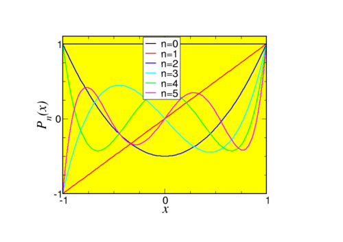
A graph of these polynomials can be found in figure 11.2 .
This work is a UK OER project as part of the Skills for Scientists project. Please contact Niels Walet for more information
 This work is licensed under a Creative Commons Attribution-Noncommercial-Share Alike 2.0 Generic License