
3.1 Linear operators
A linear operator acts on vectors in a linear vector space to give new vectors , such that 1
Example 3.1:
-
- Matrix multiplication of a column vector by a fixed matrix is a linear operation, e.g.
- Differentiation is a linear operation, e.g.,
- Integration is
linear as well,
are both linear (see example sheet).
3.1.1 Domain, Codomain and Range
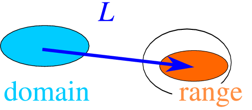
If the operators maps the vector on the vector , , the vector space of ’s (the domain) can be different from the vector space of ’s (the codomain or target). is an operator which maps the domain onto the codomain, and even though it is defined for every element of the domain, the image of the domain (called the “range of ” or the “image of ”) is in general only a subset of the codomain, see Fig. 3.1 , even though in many physical cases we shall assume that the range and codomain coincide.
Example 3.2:
-
- The operator : defined by with a fixed vector, is a linear operator.
- The matrix maps from the space of 3-vectors to the codomain of 2-vectors. The range is the 1D subset of vectors , .
- The (3D) gradient operator maps from the space of scalar fields ( is a real function of 3 variables) to the space of vector fields ( is a real 3-component vector function of 3 variables).
3.1.2 Matrix representations of linear operators
Let be a linear operator, and . Let , , …and , , …be chosen sets of basis vectors in the domain and codomain, respectively, so that
Then the components are related by the matrix relation
where the matrix is defined by
| (3.1) |
Notice that the transformation relating the components and is the transpose of the matrix that connects the basis. This difference is related to what is sometimes called the active or passive view of transformations: in the active view, the components change, and the basis remains the same. In the passive view, the components remain the same but the basis changes. Both views represent the same transformatio!
| (3.2) |
Example 3.3:
-
Find a matrix representation of the differential operator in the space of functions on the interval .
Solution:
-
Since domain and codomain coincide, the bases in both spaces are identical; the easiest and most natural choice is the discrete Fourier basis . With this choice, using and , we find
We can immediately see that the matrix representation ” ” takes the form
Matrix representation of the time-independent Schrödinger equation
Another common example is the matrix representation of the Schrödinger equation. Suppose we are given an orthonormal basis for the Hilbert space in which the operator acts. By decomposing an eigenstate of the Schrödinger equation,
in the basis as , we get the matrix form
| (3.3) |
with
This is clearly a form of Eq. ( 3.2 ).
The result in Eq. ( 3.3 ) is obviously an infinite-dimensional matrix problem, and no easier to solve than the original problem. Suppose, however, that we truncate both the sum over and the set of coefficients to contain only terms. This can then be used to find an approximation to the eigenvalues and eigenvectors. See the Mathematica notebook heisenberg.nb for an example how to apply this to real problems.
3.1.3 Adjoint operator and hermitian operators
You should be familiar with the Hermitian conjugate (also called adjoint) of a matrix, the generalisation of transpose: The Hermitian conjugate of a matrix is the complex conjugate of its transpose,
Thus
This allows us to write the inner product as a matrix product,
| (3.4) |
see Fig. 3.2 .

From the examples above, and the definition, we conclude that if is an matrix, is an one.
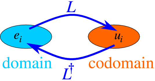
We now use our result ( 3.4 ) above for an operator, and define
where the last two terms are identical, as follows from the basic properties of the scalar product, Eq. ( 2.2 ). A linear operator maps the domain onto the codomain; its adjoint maps the codomain back on to the domain.
As can be gleamed from Fig. 3.3 , we can also use a basis in both the domain and codomain to use the matrix representation of linear operators ( 3.1 , 3.2 ), and find that the matrix representation of an operator satisfies the same relations as that for a finite matrix,
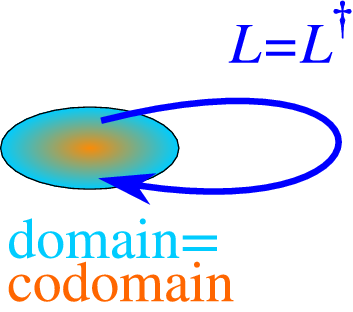
A final important definition is that of
This work is a UK OER project as part of the Skills for Scientists project. Please contact Niels Walet for more information
 This work is licensed under a Creative Commons Attribution-Noncommercial-Share Alike 2.0 Generic License