
3.4 Series solutions and orthogonal polynomials
You should all be familiar with this from the Legendre polynomials discussed in the second year math course (or see http://walet.phy.umist.ac.uk/2C1).
These functions arise naturally in the problem of the one-dimensional quantum-mechanical harmonic oscillator.
3.4.1 The quantum-mechanical oscillator and Hermite polynomials
The quantum-mechanical Harmonic oscillator has the time independent Schrödinger equation
Solutions to such equations are usually required to be normalisable,
i.e., .
Mathematical functions other than simple polynomials always act on pure numbers (since otherwise the result of the function would contain a mixture of quantities of different dimensions, as we can see by Taylor expanding). This holds here as well, and we must be able to define “dimensionless variables”. We combine all the parameters of the problem to define two scales, a harmonic oscillator length
and a scale for energy . We can then define a dimensionless coordinate and energy
In these variables the Schrödinger equation reads
| (3.12) |
Functions in must decay sufficiently fast at infinity: not all solutions to ( 3.12 ) have that property! Look at large , where , and we find that a function of the form satisfies exactly the equation
for large . Since we have neglected a constant to obtain this result, we can conclude that any behaviour of the form is allowed (since the pre-factor gives subleading terms–please check). Since the wave function must vanish at infinity, we find the only acceptable option is a wave function of the form
where does not grow faster than a power as .
The easiest thing to do is substitute this into ( 3.12 ), and find an equation for ,
| (3.13) |
This is of Sturm-Liouville form; actually we can multiply if with to find
| (3.14) |
This is a Sturm-Liouville problem, with eigenvalues . The points are singular, since vanishes. Thus is actually , as we would expect.
So how do we tackle Hermite’s equation ( 3.13 )? The technique should be familiar: we substitute a Taylor series around ,
and collect the coefficient of terms containing the same power of , and equate all these coefficients to zero
This recurrence relation can be used to bootstrap our way up from or . It never terminates, unless is an even integer. It must terminate to have the correct behaviour at infinity (like a power). We are thus only interested in even or odd polynomials, and we only have non-zero ’s for the odd part (if is odd) or even part (when is even).
If we call , with integer, the first solution is , , , …. These are orthogonal with respect to the weighted inner product
This shows that the eigenfunctions of the Harmonic oscillator are all of the form
with eigenvalue .
3.4.2 Legendre polynomials
A differential equation that you have seen a few times before, is Legendre’s equation,
| (3.15) |
Clearly are singular points of this equation, which coincides with the fact that in most physically relevant situations , which only ranges from to . As usual, we substitute a power series around the regular point , . From the recurrence relation for the coefficients,
we see that the solutions are terminating (i.e., polynomials) if for . These polynomials are denoted by . Solutions for other values of diverge at or .
Since Eq. ( 3.15 ) is of Sturm Liouville form, the polynomials are orthogonal,
As for all linear equations, the ’s are defined up to a constant. This is fixed by requiring .
Generating function
A common technique in mathematical physics is to combine all the solutions in a single object, called a “generating function”, in this case
We shall now prove that
| (3.16) |
and show that we can use this to prove a multitude of interesting relations on the way. The calculation is rather lengthy, so keep in mind where we do wish to end up: The coefficients of in Eq. ( 3.16 ) satisfy Eq. ( 3.15 ).
- First we differentiate ( 3.16 ) w.r.t. to and ,
- We then replace
on the l.h.s. of (
3.17
) by a
, multiplying both sides with
,
Equating coefficients of the same power in , we find
(3.19) - Since
times the l.h.s. of (
3.17
) equals
times the l.h.s. of (
3.18
), we can also equate the
right-hand sides,
from which we conclude that
(3.20) - Combine (
3.19
) with (
3.20
) to find
(3.21) - Let
go to
in (
3.21
), and subtract (
3.20
) times
to find
- Differentiate
this last relation,
where we have applied ( 3.20 ) one more time.
This obviously completes the proof.
We can now easily convince ourselves that the normalisation of the ’s derived from the generating function is correct,
i.e., as required.
Expansion of .
One of the simplest physical applications is the expansion of in orthogonal functions of the angle between the two vectors.
Let us first assume ,
where we have used the generating function with .
Since the expression is symmetric between and , we find the general result
where is the smaller (larger) or and .
Normalisation
When developing a general “Legendre series”, , we need to know the normalisation of . This can be obtained from the generating function, using orthogonality,
Substituting the generating function, we find
Thus
Electrostatic potential due to a ring of charge
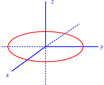
As a final example we discuss the case of a homogeneously charged ring of radius in the plane, see fig. 3.5 .
The equation to solve is , apart from on the ring itself. The problem can easily be tackled by separation of variables in polar coordinates, and we see from symmetry that the potential can only depend on and . The angular equation gives Legendre polynomials, and the radial equation is trivial to solve (it has a power of as solution), resulting in the expansion
| (3.24) |
where we have imposed the boundary condition . Actually, we can be slightly more specific and use the fact that from far away the ring looks like a point charge, for .
Now how do we determine the coefficients in ( 3.24 )? The simplest technique is based on a calculation of the potential on the positive axis. You should have derived the result before (it is a standard example in basic electrostatics)
This can easily be expanded in powers of , and if we use we get
Since on the positive axis and , we conclude that
3.4.3 Bessel functions and the circular drum
Bessel’s equation of order takes the form
This equation has a regular singular point at , and the point is regular. It is thus not of Sturm-Liouville form, without additional boundary conditions (see below).
The solutions can be found in many places: we substitute a generalised power series around ,
From the index equation (lowest power in ) we find ; this leads to two independent solutions if is not a half-integer. The recurrence relations are
The main result are the Bessel functions (regular solutions) for ,
The simplest use of these regular solutions is for example in the caculation of the modes in a circular drum. With we find that
| (3.25) |
with the explicit boundary condition and the implicit boundary condition is finite. With these conditions we have an Sturm-Liouville problem!
We can move into the variable by using the transformation
which turns the equation into Bessel’s equation of order . Thus
with the boundary condition
If we are given the zeroes of , we find that
We tabulate the zeroes of in Tab. 3.2 .
|
|
|
|
|
|
| 1. | 2.5387339670887545 | 4.5605686201597395 | 7.038761346947694 | |
| 5.2689404316052215 | 8.510612772447574 | 12.25103245391653 | 16.47492803352439 | |
| 12.949091948711432 | 17.89661521491159 | 23.347115194125884 | 29.291025900157134 | |
| 24.042160379641803 | 30.696015647982048 | 37.85459961832423 | 45.51139388242945 | |
| 38.5483546692039 | 46.90868597534144 | 55.77464019991307 | 65.14149844841049 | |
| 56.46772471517244 | 66.53458968257806 | 77.10759560464034 | 88.18317085819912 | |
| 77.80028714289776 | 89.5737132318928 | 101.85360724822897 | 114.63717276642296 | |
| 102.54604874469128 | 116.02605067898523 | 130.01274014487907 | 144.50386866809274 | |
| 130.70501270873422 | 145.89159908441692 | 161.58502760864766 | 177.78345128038563 | |
| 162.2771806904681 | 179.1703568603581 | 196.57048815295988 | 214.47603043403043 |
This work is a UK OER project as part of the Skills for Scientists project. Please contact Niels Walet for more information
 This work is licensed under a Creative Commons Attribution-Noncommercial-Share Alike 2.0 Generic License