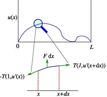
Figure 4.1: The balance of forces in a driven string
The Green function technique is used to solve differential equations of the form
|
({L}_{x}u)(x) = f(x)\qquad \text{plus boundary conditions}
| (4.1) |
where {L}_{x} is a linear hermitian operator with specified boundary conditions and f(x) is a given “source term”. We shall normally suppress the subscript x on L.
The solution of (4.1) can always be written as
|
u(x) =\mathop{ \mathop{\mathop{∫
}\nolimits }}\nolimits dx'\kern 1.66702pt G(x,x')f(x'),
| (4.2) |
where the Green function G(x,x') is defined by
|
LG(x,x') = δ(x − x')\qquad \text{plus boundary conditions},
| (4.3) |
where L acts on x, but not on x'. We also have the same boundary conditions as before! The proof is straightforward:
Note by solving this equation, one obtains the solution of (4.1) for all possible f(x), and thus it is very useful technique to solve inhomogeneous equations where the right-hand side takes on many different forms.
In your physics courses you have already been exposed to a Green function, without it ever being made explicit. The problem of interest is the determination of the electrostatic potential Φ(x) for a static charge distribution ρ(x). From \mathop{∇}⋅E = ρ∕{ϵ}_{0} and E = −\mathop{∇}Φ we can easily show that
|
{\mathop{∇}}^{2}Φ(x) = −ρ(x)∕{ϵ}_{
0},
| (4.5) |
with the boundary condition that Φ(x) → 0 as |x|→∞.
For a point charge q at position x', Eq. (4.5) becomes
[The notation {δ}^{(3)}(x) stands for the 3D δ function δ(x)δ(y)δ(z).] We all know the solution, which is Coulomb’s law,
In other words, the Green function G which solves
is
|
G(x,x') = − {1\over
4π} {1\over
|x−x'|}.
| (4.6) |
This leads to the well known superposition principle for a general charge distribution,
This is usually derived using the statement that each “small charge” δQ(x') = {d}^{3}x'ρ(x') contributes {1\over 4π{ϵ}_{0}} {δQ(x')\over |x−x'|} to the potential Φ, and we simply superimpose all these contributions.
For operators where we know the eigenvalues and eigenfunctions, one can easily show that the Green functions can be written in the form
This relies on the fact that {u}_{n}(x) is a complete and orthonormal set of eigenfunctions of L, obtained by solving
|
L{u}_{n}(x) = {λ}_{n}{u}_{n}(x),
| (4.7) |
where we have made the assumption that there are no zero eigenvalues.
If there are zero eigenvalues–and many important physical problems have “zero modes”–we have to work harder. Let us look at the case of a single zero eigenvalue, {λ}_{0} = 0. The easiest way to analyse this problem is to decompose u(x) and f(x) in the eigenfunctions,
We know that {d}_{n} = ({u}_{n},f), etc.
Now substitute (4.8) into (4.7) and find
Linear independence of the set {u}_{n} gives
and of most interest
|
0 = {c}_{0}{λ}_{0} = {d}_{0}.
| (4.9) |
Clearly this equation only has a solution if {d}_{0} = 0. In other words we must require that ({u}_{0},f) = 0, and thus the driving term f is orthogonal to the zero mode. In that case, {c}_{0} is not determined at all, and we have the family of solutions
Here
with
Consider a string with fixed endpoints (such as a violin string) driven by an oscillating position-dependent external force density,
If we now consider a small section of the string, see Fig. 4.1, and assume small displacements from equilibrium, we can use the fact that the tension in the string and its density are constant, and we can use the tranvserse component of Newton’s equation for teh resulting transverse waves,
Using a Taylor series expansion of u and taking the limit dx ↓ 0, we find
We know how such a problem works; there is a transient period, after which a steady state oscillations is reached at the driving frequency, u(x,t) = v(x)\mathop{sin}\nolimits ωt, i.e.,
Using this relation, we obtain a complicated equation for the steady state amplitude v(x),
This can be simplified by writing {k}^{2} = ρ{ω}^{2}∕T and f(x) = F(x)∕T,
|
v'' + {k}^{2}v = f(x),
| (4.10) |
with boundary conditions v = 0 at x = 0 and x = L.
Now follow the eigenstate method for Green functions. First we must solve
If we write this as {v}_{n}'' = ({λ}_{n} − {k}^{2}){v}_{n}, we recognise a problem of the simple form y'' = ky, which is solved by functions that are either oscillatory or exponential. The boundary conditions only allow for solutions of the form {v}_{n} = \sqrt{2∕L}\mathop{sin}\nolimits {k}_{n}x with {k}_{n} = nπ∕L. From this we conclude that {λ}_{n} = {k}^{2} − {k}_{n}^{2}, and thus
The solution becomes
where
Clearly, we have not discussed the case where takes on the values k = {k}_{m}, for any integer m ≥ 1. From the discussion before we see that as k approaches such a point the problem becomes more and more sensitive to components in f of the mth mode. This is the situation of resonance, such as the wolf-tone of string instrument.
In this method for solving second order equations of the form
one
see below for an explanation.
Let us illustrate the method for the example of the driven vibrating string discussed above,
and
|
\left ( {{d}^{2}\over
d{x}^{2}} + {k}^{2}\right )G(x,x') = δ(x − x'),
| (4.11) |
with boundary conditions G(x,x') = 0 if x = 0,L. This can also be given a physical interpretation as the effect a point force acting at x = x'.
We first solve the problem
|
{{∂}^{2}\over
∂{x}^{2}}G(x,x') + {k}^{2}G(x,x') = 0.
|
in the two regions x < x', x > x', which differ in boundary conditions,
since G(0,x') = 0 falls within this domain.
since G(L,x') = 0 falls within this domain.
We now require that G(x,x') is continuous in x at x = x' (a point force doesn’t break the string), and that {∂}_{x}G(x,x') is discontinuous at x = x' (since a point force “kinks” the string).
To find this discontinuity, we integrate (4.11) over x around x' (where ϵ is a very small number)
or
In the limit ϵ → 0 we find that
From the form of G derived above, we conclude that
with as solution (as can be checked using the formula \mathop{sin}\nolimits A\mathop{cos}\nolimits B +\mathop{ cos}\nolimits A\mathop{sin}\nolimits B =\mathop{ sin}\nolimits (A + B))
Taking this together we find
Note the symmetry under interchange of x and x', which is a common feature on Green functions.
As a challenge problem, you may wish to check that this form is the same as the one derived by the eigenfunction method in the previous section (see also the mathematica based coursework).