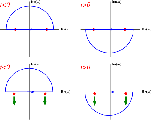
Figure 4.2: The contours used in the
ω
integral (4.19).
In electromagnetism, you may have met the equations for the scalar potential Φ and vector potential A, which in free space are of the form
These equation are satisfied for the “gauge choice” \mathop{∇}⋅A = 0, the Coulomb or radiation gauge.
As usual we can analyse what happens with external charge and current distributions, where the potentials satisfy
|
□Φ = {ρ(r,t)\over
{ϵ}_{0}} ,\qquad □A = {μ}_{0}j(r,t).
| (4.14) |
Since we would like to know what happens for arbitrary sources, we are immediately led to the study of the Green function for the D’Alembertian or wave operator □,
|
□G(r,t;r',t) = δ(r −r')δ(t − t').
|
The boundary conditions are
For Galilean invariant problems, where we are free to change our origin in space and time, it is simple to show that the Green function only depends on (r −r') and t − t' ,
To obtain the functional form of G it is enough to solve for r' = 0, t' = 0, i.e.
|
\left ( {1\over {
c}^{2}} {{∂}^{2}\over
∂{t}^{2}} −{\mathop{∇}}^{2}\right )G(r,t) = δ(r)δ(t).
| (4.15) |
This standard method for time dependent wave equations is in several steps: First define the Fourier transform of G
and solve for the Fourier transform \tilde{G}(k,ω) by substituting the second of these relations into Eq. (4.15): This equation becomes
If we now equate the integrands, we find that
We now substitute \tilde{G}(k,ω) back into (4.16)
The {d}^{3}k part of the integral (4.17) is of the generic form
Integrals of this type can be dealt with in a standard way: We are free to choose the {k}_{3} axis to our benefit, since we integrate over all k, and this preferred direction makes no difference to the value of the integral. Thus, we choose the {k}_{3}-axis parallel to r, and find
Note the trick used to transform the penultimate line into the last one: we change the second term in square brackets into an integral over (−∞,0].
We can now apply this simplification to (4.17) to find
We now tackle the ω integral,
|
{\mathop{\mathop{\mathop{∫
}\nolimits }}\nolimits }_{−∞}^{∞}{dω\over
2π}\kern 1.66702pt {{e}^{−iωt}\over {
ω}^{2} − {c}^{2}{k}^{2}}.
| (4.19) |
The problem with this integrand is that we have poles at ω = ±ck on the real axis, and we have to integrand around these in some way. Here the boundary conditions enter. We shall use contour integration by closing off the integration contour by a semicircle in the complex ω plane. The position of the semicircle will be different for positive and negative t: Look at
|
ω = R{e}^{iϕ},
|
where R is the radius of the semicircle (which we shall take to infinity), and ϕ is the variable that describes the movement along the semicircle. We find that
|
\mathop{exp}\nolimits [−iωt] =\mathop{ exp}\nolimits [−iRt\mathop{cos}\nolimits ϕ]\mathop{exp}\nolimits [Rt\mathop{sin}\nolimits ϕ].
|
Since we want to add a semicircle without changing the integral, we must require that
|
\mathop{exp}\nolimits [Rt\mathop{sin}\nolimits ϕ] → 0\text{ as }R →∞,
|
so that no contribution is made to the integral. This occurs if t\mathop{sin}\nolimits ϕ < 0. Thus, if t < 0, we close the contour in the upper half plane, and if t > 0 in the lower one, see Fig. 4.2.
Now we have turned our ω integral into a contour integral, we need to decide how to deal with the poles, which lie on the real acis. Our time boundary condition (causality) states that G = 0 if t < 0, and thus we want to move the poles to just below the contour, as in the second part of Fig. 4.2, or by shifting the integration up by an infinitesimal amount above the real axis (these two ways of doing the integral are equivalent). The integral for t > 0 can then be done by residues, since we have two poles inside a closed contour. Note that the orientation of the contour is clockwise, and we just have a minus sign in the residue theorem,
Here {R}_{±} is the residue of the poles (the “strength” of the pole),
and we thus find that
If we substitute this into (4.18), we find that (t > 0!)
We discard the second delta function above, since its argument r + ct > 0 if t > 0, and thus the δ function is always zero.
If we now reinstate t' and r' using Galilean invariance, we find that
|
G(r,t;r',t) = {c\over
4π|r −r'|}δ{\bigl (|r −r'|− c(t − t')\bigr )}.
| (4.20) |
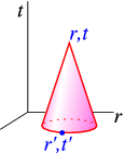
For reasons that will become clear below, this is called the retarded Green function. It vanishes everywhere except on the backward light cone, |r −r'| = c(t − t'), see Fig. 4.3.
Two special cases can be obtained simply:
using
The δ function selects those points on the path followed by the charge that intersect the light-cone with apex r,t at a time s(t'),t'.
Green functions for wave equations in (2+1) dimensions can be solved directly by the Fourier transform method, or, if you know the result in (3+1) dimensions, they can also be obtained by “integrating out” the extra dimensions:
|
{G}^{(2)}(x − x',y − y',t − t') =\mathop{ \mathop{\mathop{∫
}\nolimits }}\nolimits dz'\kern 1.66702pt G(r,t;r',t')
| (4.21) |
for t > t'.
This can be checked quite simply. From
|
□G(r,t;r',t) = δ(r −r')δ(t − t').
|
We find that
|
\mathop{\mathop{\mathop{∫
}\nolimits }}\nolimits dz'\kern 1.66702pt □G(r,t;r',t') =\mathop{ \mathop{\mathop{∫
}\nolimits }}\nolimits dz'\kern 1.66702pt δ(r −r')δ(t − t').
|
If we now swap differentiation and integration, we get
|
□\mathop{\mathop{\mathop{∫
}\nolimits }}\nolimits dz'\kern 1.66702pt G(r,t;r',t') = δ(x − x')δ(y − y')δ(t − t').
|
Since \mathop{\mathop{\mathop{∫ }\nolimits }}\nolimits dz'\kern 1.66702pt G(r,t;r',t') = {G}^{(2)}(x − x',y − y',t − t') is independent of z, we find that {∂}_{z}^{2}{G}^{(2)} = 0, and thus {G}^{(2)} is indeed the Green function for the two-dimensional wave equation.
From equation (4.20) we find
|
\mathop{\mathop{\mathop{∫
}\nolimits }}\nolimits dz'\kern 1.66702pt {c\over
4π|r −r'|}δ{\bigl (|r −r'|− c(t − t')\bigr )}
|
Integrate using the delta function, which is nonzero at {z'}_{±} = z ±\sqrt{{c}^{2 } {(t − t')}^{2 } − {(x − x')}^{2 } − {(y − y')}^{2}}, and thus
Both poles give the same contribution, and the retarded Green function is thus
|
{G}^{(2)}(x−x',t − t') = {c\over
2π} {1\over {
({c}^{2}{(t − t')}^{2} −|x−x'{|}^{2})}^{1∕2}}
| (4.22) |
for t > t' , where x is a 2-dimensional space vector x = (x,y). In contrast to the 3+1 case, this is non-vanishing in the whole of the backward light-cone, not just on it!