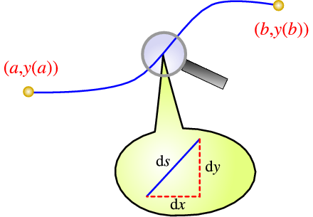
Figure 5.1: The distance between two points along a path connecting two fixed points
Let us look at a few special cases for the functional I defined in (5.1).
We first consider the case F(y(x),y'(x),x) = F(y'(x),x), and thus independent of y. The Euler-Lagrange equation,
has the simple solution
|
{∂F\over
∂y'(x)} = \text{constant}.
| (5.4) |
This equation is called the “first integral” of the problem.
Example 5.2:
Show that the shortest distance between any two fixed points (in 2D space, for simplicity) is along a straight line.
Solution:
We parametrise the curve connecting the two points by (x,y(x)) (which assumes each value x only occurs once, and we thus only look at a–sensible–subclass of paths). The endpoints (a,y(a)) and (b,y(b)) are fixed. If we take a small step along the line, the distance travelled is
Thus
The total path length is thus the functional
which is of the form investigated above. Thus
It is not too hard to solve this equation, by squaring both sides,
We can determine c and d from the boundary conditions
If F(y,y',x) = F(y,y'), independent of x, we proceed in a slightly different way. We combine the Euler-Lagrange equation
with an explicit differentiation of F,
to find
Combining left-hand and right-hand sides, we find
We thus conclude that for F[y,y'] (i.e., no explicit x dependence in the functional) we have the first integral
|
\class{boxed}{ F − y' {∂F\over
∂y'(x)} = \text{constant}\quad . }
| (5.5) |
Example 5.3:
Fermat’s principle of geometrical optics states that light always travels between two points along the path that takes least time, or equivalently which has shortest optical path length (since time is pathlength divided by the speed of light). Show that this implies Snell’s law.
Solution:
Following notations as for the shortest path problem above, we find that the travel time of light along an arbitrary path y(x) is
or in terms of the optical path
We have assumed that n(x,y) = n(y). Its correctness depends on both path and arrangement of the problem.
We now use the result (5.5) from above, and find with F = n(y(x))\sqrt{1 +{ y' }^{2}} that
Thus
|
\class{boxed}{n(y) = \text{const}\sqrt{1 +{ y' }^{2}}\quad . }
| (5.6) |
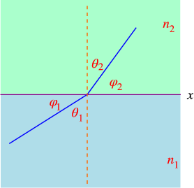
Now consider areas where n(y) is constant. The problem turns into the least distance problem discussed above, and we find that in such an area the optical path becomes a straight line. We now assume two such areas, with index of refraction {n}_{1} below the x axis, and {n}_{2} above, see Fig. 5.2. As usual it is easy to see that y'(x) =\mathop{ tan}\nolimits ϕ, and from
we conclude from Eq. (5.6) that n\mathop{cos}\nolimits ϕ = \text{constant}. Thus
and using \mathop{cos}\nolimits ϕ =\mathop{ cos}\nolimits ({π\over 2} − θ) =\mathop{ sin}\nolimits θ we get
|
\class{boxed}{{n}_{1}\mathop{ sin}\nolimits {θ}_{1} = {n}_{2}\mathop{ sin}\nolimits {θ}_{2}, }
|
i.e., we have proven Snell’s law.
Let’s look at one more related problem
Example 5.4:
The brachistochrone is the curve along with a particle slides the fastest between two points under the influence of gravity; think of a bead moving along a metal wire. Given two fixed endpoints, A = (0,0) and a second point B, find the brachistichrone connecting these points.
Solution:
We find for the travel time
which has to be a minimum. From energy conservation we get
and as before
Taking all of this together
|
T[y] ={\mathop{ \mathop{\mathop{∫
}\nolimits }}\nolimits }_{0}^{b}{\left ({1 +{ y'}^{2}\over
2gy} \right )}^{1∕2}dx.
| (5.7) |
We now drop the factor 2g from the denominator, and minimise
Since F ={ \left ({1+{y'}^{2}\over y} \right )}^{1∕2} has no explicit x dependence, we find
i.e.,
Substituting a convenient value for the constant, we find
|
\class{boxed}{y(1 +{ y'}^{2}) = 2R, }
|
which is the equation for a cycloid. To solve this, we write y' =\mathop{ cot}\nolimits (ϕ∕2), which now leads to
and
|
y(ϕ) = 2R∕(1 +{ y'}^{2}) = 2R{\mathop{sin}\nolimits }^{2}(ϕ∕2) = R(1 −\mathop{ cos}\nolimits ϕ).
| (5.8) |
That would be fine if we knew also x(ϕ), so we can represent the curve by a parametric plot! We have from (5.8)
Thus using Eq. (5.8) we get x = R(ϕ −\mathop{ sin}\nolimits ϕ) + C. Imposing the condition that the curve runs through (0,0), we find
|
\class{boxed}{x = R(ϕ −\mathop{ sin}\nolimits ϕ),\qquad y = R(1 −\mathop{ cos}\nolimits ϕ). }
|
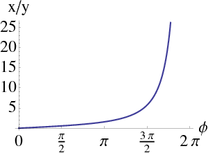
We determine R and an angle {ϕ}_{0} from the conditions
This has multiple solutions. In order to cover all points with positive x∕y once, we need to require 0 < ϕ < 2π, see Fig. 5.3.
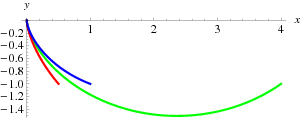
Once we have fixed the range of ϕ, we can then solve for the brachystochrone, see Fig. 5.4 for a few examples.
So what is the value of the travel time? Substituting the solution into Eq. (5.7) we get