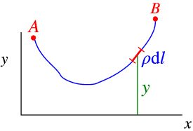
Figure 5.7: The isoperimetric problem.
It is quite common that we have subsidiary conditions on a minimisation problem, i.e., we want to know the minimum provided that certain other conditions hold. Let us first analyse this problem for ordinary functions first
To find the stationary points of a function f(x) subject to constraints {g}_{k}(x) = 0, (k = 1,2,\mathop{\mathop{…}}), we can solve an extended problem and find the unconstrained stationary points of the extended functional
|
F(x,{λ}_{1},{λ}_{2},\mathop{\mathop{…}}) = f(x) − {λ}_{1}{g}_{1}(x) − {λ}_{2}{g}_{2}(x) −\mathop{\mathop{…}},
| (5.18) |
w.r.t to x and {λ}_{i}.
Let’s look at a somewhat explicit example. We wish to minimise a function f(x,y) subject to a single constraint g(x,y) = 0. We thus need to minimise the extended function
and find
The last line clearly states that the constraint must be implemented. The new terms (proportional to λ) in the first two lines say that a constrained minimum is reached when the gradient of the function is parallel to the gradient of the constraint. This says that there is no change in the function, unless we violate our constraint condition–clearly a sensible definition of a stationary point.
Example 5.10:
Find stationary points of f(x,y) under the subsidiary condition {x}^{2} + {y}^{2} = 1.
Solution:
Look for stationary points of
which are given by the solution(s) of
The first two conditions give {x}^{2} = {y}^{2}, and from the constraint we find (x,y) = (±1∕\sqrt{2},±1∕\sqrt{2}). The values of λ associated with this are λ = ±1∕2.
We look for stationary points of I[y] subject to a constraint J[y] = C, (can also be multiple constraints) where I, J are given functionals of y(x) and C is a given constant.
To do this: we solve for the stationary points of an extended funtional,
|
K[y,λ] = I[y] − λ(J[y] − C)\quad ,
| (5.19) |
with respect to variations in the function y(x) and λ. We then have
which can be dealt with as an unconstrained variational problem. Its solution can be slightly tricky; one way is to solve the problem
for fixed λ to find y(x) as a function of λ, and then use the constraint J[y] = C to find the allowed value(s) of λ, and thus the solution.
Example 5.11:
Find a closed curve of fixed length L = 2πl
which encloses the maximum area A.
(The isoperimetric problem, see Fig. 5.7.)
Solution:
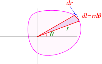
Describe the curve in polar coordinates by (θ,r(θ)), assuming the origin lies within the curve. We then find that
We now need to find stationary points of
Minimising with respect to r(θ), we find a problem where there is no explicit dependence of the function we usually call “F” on θ, and thus
Explicitly,
together with the constraint
Unfortunately, this equation is not easy to solve in general, but we can guess one solution: Look at λ = 0 when we find r = l, K = {l}^{2}∕2. This describes a circle through the origin. By translational invariance we see any other circle also satisfies this condition.
Example 5.12:
What is the equilibrium curve for a flexible “chain” of length l and density ρ per unit length, when we hang it between two points A and B. (The catenary, see Fig. 5.8.)
Solution:
We need to minimise the gravitational potential energy
subject to the constraint of constant length L[y] = l, with
Thus we need to find stationary points of G[y] = E[y] − λ(L[y] − l).
As usual the variation with respect to y is simple, since the integrand
has no explicit dependence on x we can use the first integral,
or explicitly,
This can be solved by making a shift on y,
The new function u satisfies
Now use u = α\mathop{cosh}\nolimits w, du = α\mathop{sinh}\nolimits w\kern 1.66702pt dw to find
The three constants α, {x}_{0} and λ are determined by the condition that line goes through A and B and has length
The point {x}_{0} is where the curve gets closest to the ground. If y(a) = y(b), {x}_{0} = (a + b)∕2 by symmetry.
A good demonstration can be found on ”Catenary: The Hanging Chain” on The Wolfram Demonstrations Project.
Consider the eigenvalue equation for the function u(x)
|
Lu = λρu\quad ,
| (5.21) |
where L is an Hermitian operator, ρ(x) is a positive, real weight function. We now look for the stationary points of
|
I[u] =\mathop{ \mathop{\mathop{∫
}\nolimits }}\nolimits dτ\kern 1.66702pt {u}^{∗}Lu
| (5.22) |
subject to the normalisation constraint
|
\mathop{\mathop{\mathop{∫
}\nolimits }}\nolimits dτ\kern 1.66702pt ρ{u}^{∗}u = 1.
| (5.23) |
We first look for an unconstrained stationary point of
and vary λ to obtain a solution that satisfies the constraint. We get
where we have used hermiticity of the operator L.
A key difference with the previous examples is that we have a complex function u, and any variation thus falls into two parts,
The real and imaginary parts are independent small functions, i.e., we can vary those independently. In the same way we can conclude that the alternative orthogonal combination of these two variations provided by δu and δ{u}^{∗} vary independently, so we can select either of the two terms above, since they must both be zero independently. The function multiplying δ{u}^{∗} must thus satisfy
which shows u is an eigenfunction of L. We conclude that the stationary points are the eigenfunctions u = {u}_{0},{u}_{1},\mathop{\mathop{…}} and the corresponding values of λ are the eigenvalues {λ}_{0},{λ}_{1},\mathop{\mathop{…}}.
Now suppose that there is a minimum eigenvalue {λ}_{0}. This implies that for a normalised u, I[u] ≥ {λ}_{0}. We show below how we can use that to our benefit.
Suppose the function {u}_{0} gives the minimum of
subject to the constraint
Now suppose {v}_{0} gives the unconstrained minimum of
|
K[v] = {\mathop{\mathop{\mathop{∫
}\nolimits }}\nolimits dτ{v}^{∗}Lv\over
\mathop{\mathop{\mathop{∫
}\nolimits }}\nolimits dτ{v}^{∗}ρv} .
| (5.24) |
Theorem 5.1. The unconstrained minimum of K[v] and the constrained minimum of I[u] with the normalisation constraint are identical.
Proof.
(The last inequality holds if {v}_{0} is the minimum of K). Now find a similar relation for I. Define N = \mathop{\mathop{\mathop{∫ }\nolimits }}\nolimits dτ{v}_{0}^{∗}ρ{v}_{0} and {w}_{0} = {v}_{0}∕\sqrt{N}, then
Thus K[{v}_{0}] = I[{u}_{0}], and unless there are degenerate minima, {w}_{0} = {u}_{0}. □
This technique is very commonly used in quantum mechanics, where we then replace the functional dependence with a parametrised dependence by choosing a set of wave functions depending on set of parameters. In this case L = H, ρ = 1 and u = ψ.
Example 5.13:
Find an approximation to the ground state of the quartic anharmonic oscillator
of the form ψ(x) =\mathop{ exp}\nolimits (−α{x}^{2}∕2).
Solution:
The normalisation integral is
By differentiating both sides w.r.t. α, we get two more useful integrals,
Thus the expectation value of the Hamiltonian requires the derivative
Thus the denominator of the variational functional becomes
And thus
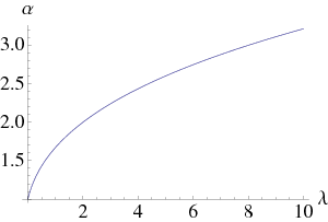
Minimising w.r.t. α, we find
This equation can be solved in closed form, but is rather complicated. We find that α increases with λ, see Fig. 5.9.