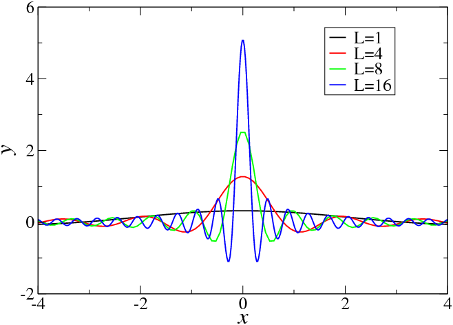
Figure 2.1: A sketch of {1\over
2π} {2\over
x}\mathop{ sin}\nolimits (Lx)
for a few values of L.
This function converges to a Dirac delta function
The Dirac delta function δ(x) is defined by the “reproducing” property, i.e.,
|
\mathop{\mathop{\mathop{∫
}\nolimits }}\nolimits dx'\kern 1.66702pt δ(x − x')f(x') = f(x)
|
for any function f(x).6 This is equivalent to the following explicit definition (further forms are discussed in the Mathematica examples), see also Fig. 2.1.
|
δ(x) = {1\over
2π}{\mathop{\mathop{\mathop{∫
}\nolimits }}\nolimits }_{−∞}^{∞}dz\kern 1.66702pt {e}^{izx} ≡ {1\over
2π}{\mathop{lim}}_{L→∞}{\mathop{\mathop{\mathop{∫
}\nolimits }}\nolimits }_{−L}^{L}dz\kern 1.66702pt {e}^{izx} = {1\over
2π}{\mathop{lim}}_{L→∞}{2\over
x}\mathop{sin}\nolimits (Lx)\quad .
|
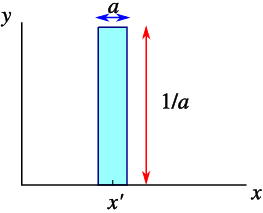
It is often useful to think of the δ function as the limit of a simple function, and one example is an infinitely narrow spike, as in Fig. 2.2 for a → 0.
Since integration with the δ function “samples” f(x') at the single point x' = x, we must conclude that
The area under the δ function is 1, as can be seen from taking f(x') = 1. Combining the last two results leads to an interesting expression for the area under the curve,
A very useful relation is obtained when we scale the variables in the delta function (y = ax)
|
{\mathop{\mathop{\mathop{∫
}\nolimits }}\nolimits }_{−∞}^{∞}dx'\kern 1.66702pt δ(a(x − x'))f(x') =\mathop{ sign}\nolimits (a){1\over
a}{\mathop{\mathop{\mathop{∫
}\nolimits }}\nolimits }_{−∞}^{∞}dy'\kern 1.66702pt δ(y − y')f(y'∕a) = {f(y∕a)\over
|a|} = {f(x)\over
|a|} .
|
We can interpret this is as the contribution from the slope of the argument of the delta function, which appears inversely in front of the function at the point where the argument of the δ function is zero. Since the δ function is even, the answer only depends on the absolute value of a. Also note that we only need to integrate from below to above the singularity; it is not necessary to integrate over the whole infinite interval.
This result can now be generalised to a δ-function with a function as argument. Here we need to sum over all zeroes of the function inside the integration inetrval, and the quantity a above becomes the slope at each of the zeroes,
|
{\mathop{\mathop{\mathop{∫
}\nolimits }}\nolimits }_{a}^{b}dx\kern 1.66702pt g(x)\kern 1.66702pt δ\left (f(x)\right ) ={ \mathop{∑
}}_{i}{\left ({g(x)\over
\left |{df\over
dx}\right |}\right )}_{x={x}_{i}}
|
where the sum extends over all points {x}_{i} in \left ]a,b\right [ where f({x}_{i}) = 0.
Example 2.6:
Calculate the integral
Solution:
Let us first calculate the zeroes of {x}^{2} − {c}^{2}{t}^{2}, x = ±ct.. The derivative of {x}^{2} − {c}^{2}{t}^{2} at these points is ± 2ct, and thus
Integrals such as these occur in electromagnetic wave propagation.