
To be used in future
Prev Section 3.3: Consequences for Quantum Mechanics
Up Chapter 3: Symmetries
Chapter 4: Charged Particles and Electromagnetic Fields Next
3.4 Unitary operators↓
3.4.1 Exponent of generators↓
Once we know what the generators are, we can try and take many small steps to make one big step. Finding explicit expressions will rely on the basic formula from calculus
The proof of this relations is simple; we use the binomial expansion and find
3.4.2 Unitarity
A very important class of operators (transformations) in quantum mechanics are those that preserve the norm of a wave function, or slightly more generally the scalar product (overlap) between any two wave functions. Let
be one such operator. By definition the transformed ket becomes
and thus
if the scalar product is preserved. Since we require this to hold for any
and
, we find
or
3.4.2.1 Unitarity of the transformation operators
We can show that any symmetry transformation that changes space in such a way as to leave the volume element invariant has an operator representation that is unitary: Consider the scalar product
We find that if for any symmetry operation
where the volume element satisfies
(the small volume element
gets transformed into a volume of equal size) we get
We also know that
Since
and
are arbitrary, we have
3.4.3 Translation in space↓↓
We start by taking dividing a translation into many smaller translations
It is easy to show that
and thus
, which shows that this is a unitary (norm preserving) operator. It is actually quite straightforward (and useful) to show that any operator of the form
with
a Hermitian operator is unitary [see example sheet].
3.4.4 Translation in time↓↓
It is even more useful to do this for time translations
The operator we have found over here is called the time evolution operator↓. Once again, it is trivially unitary.
3.4.5 Rotations↓↓
By now it should have become second nature to show that
This obviously unitary.
For a problem with rotational symmetry, we normally usually use a basis of the form
where
and
is a place holder for the remaining quantum numbers needed to specify the states. The choice of rotation angles we have made is not very well matched to this choice; we shall make an equivalent choice below.
3.4.5.1 ↓Euler angles
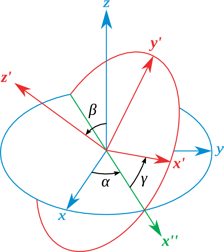
The axis/angle representation is not very well chosen for the basis (↓). Fortunately there is an alternative representation of rotations due to Euler that is commonly used because it has many useful properties, and also helps in this case. In this parametrisation we write a rotation as a product of three simple rotations. We first perform a rotation about the
axis with angle
(
). This moves the
and
axes to point in a new direction in the
plane. Then perform a rotation over an angle
(
) along the new
axis. Finally, perform a rotation about an angle
(
) along the new
axis. [J] [J] These angles are called
,
and
in many textbooks; we shall not use this notation, since it tends to lead to confusion with the polar angles. If we perform the transformation
the operator implementing this transformation can clearly be written as
Note the change in order! This is due to the fact that
3.4.5.2 Representation matrices↓
If we look at the matrix elements of
in a basis of states
(i.e., these are purely angular states, we suppress any additional labels. In polar angles we have
) we find that
where we use the fact that
cannot change the value of
(since
). Clearly what remains now is the much simpler task to find the matrices
that only depend on a single angle, see below for a simple example.
3.4.5.3 Angular momentum states and ladder operators↓
In order to work out some of the algebraic details of the angular momentum states it is convenient to change from
and
to the ladder operators
These have the nice property
We find that for the states
satisfying
we have
Thus
where
is an as yet undetermined normalisation constant. If we write
this can be used to show that (using the “obvious” relation
)
and similar for
. We cannot fix the phase of
: A little thought shows this can be freely chosen, since it corresponds to a phase choice for the angular momentum eigenstates. We use
Rewriting
, we can now find the basic ingredients to evaluate the exponential of
in the expression for
.
3.4.5.4 ↓
It is instructive to look at the case
. We quickly find that
and thus, if we order the basis as
we have the matrix representation↓ for
for
Question: What must be the eigenvalues of the matrix? Check that this is indeed the case.
We can now calculate
This could get complicated, but fortunately
and
Thus all odd powers and all even powers of the matrix are equal--apart from the “zeroth power”. We thus find that
Thus
3.4.5.5 Spin↓
We have not yet looked at the thorny issue of intrinsic quantum numbers and their symmetries. One place where we can relatively straightforwardly do that is for angular momentum. We know that for a system with spin, the total angular momentum↓↓
is conserved, and we can immediately generalise the transformation (↓) to
What happens if we look at that case
,
, i.e., a pure spin
particle? It is relatively easy to evaluate the values of
using the Pauli matrix
(details on example sheet);
The most interesting fact is what happens under a
rotation. For ease of calculation take it along the
-axis, and we find that
in other words, a spin
state goes to minus itself under a
space rotation! ↓
This work is a Open Educational Resource. Please contact Niels Walet for more information, or further licensing.
 This work is licensed under a Creative Commons Attribution-Noncommercial-Share Alike 3.0 Generic License