6.2 New variables

In order to understand the solution in all mathematical details we make a change of variables

w = x + ct,\quad z = x − ct.
(6.2)

We write u(x,t) =\bar{ u}(w,z). We find

\begin{eqnarray} {∂u\over ∂x}& =& {∂\bar{u}\over ∂w} {∂w\over ∂x} + {∂\bar{u}\over ∂z} {∂z\over ∂x} = {∂\bar{u}\over ∂w} + {∂\bar{u}\over ∂z}, %& \\ {{∂}^{2}u\over ∂{x}^{2}}& =& {{∂}^{2}\bar{u}\over ∂{w}^{2}} + 2 {{∂}^{2}\bar{u}\over ∂w∂z} + {∂\bar{u}\over ∂z}, %& \\ {∂u\over ∂t} & =& {∂\bar{u}\over ∂w} {∂w\over ∂t} + {∂\bar{u}\over ∂z} {∂z\over ∂t} = c\left ( {∂\bar{u}\over ∂w} −{∂\bar{u}\over ∂z}\right ),%& \\ {{∂}^{2}u\over ∂{t}^{2}} & =& {c}^{2}\left ( {{∂}^{2}\bar{u}\over ∂{w}^{2}} − 2 {{∂}^{2}\bar{u}\over ∂w∂z} + {∂\bar{u}\over ∂z}\right ) %&(6.3) \\ \end{eqnarray}

We thus conclude that

{{∂}^{2}u\over ∂{x}^{2}}(x,t) − {1\over { c}^{2}} {{∂}^{2}u\over ∂{t}^{2}} (x,t) = 4 {{∂}^{2}\bar{u}\over ∂w∂z} = 0
(6.4)

An equation of the type {{∂}^{2}\bar{u}\over ∂w∂z} = 0 can easily be solved by subsequent integration with respect to z and w. First solve for the z dependence,

{∂\bar{u}\over ∂w} = Φ(w),
(6.5)

where Φ is any function of w only. Now solve this equation for the w dependence,

\bar{u}(w,z) =\mathop{ \mathop{\mathop{∫ }\nolimits }}\nolimits Φ(w)dw = F(w) + G(z)
(6.6)

In other words,

\class{boxed}{ u(x,t) = F(x + ct) + G(x − ct), }

with F and G arbitrary functions.

6.2.1 Infinite String

This equation is quite useful in practical applications. Let us first look at how to use this when we have an infinite system (no limits on x). Assume that we are treating a problem with initial conditions

u(x,0) = f(x),\kern 2.77695pt \kern 2.77695pt {∂u\over ∂t} (x,0) = g(x).
(6.7)

Let me assume f(±∞) = 0. I shall assume this also holds for F and G (we don’t have to, but this removes some arbitrary constants that don’t play a rôle in u). We find

\begin{eqnarray} F(x) + G(x)& =& f(x),%& \\ c(F'(x) − G'(x))& =& g(x). %&(6.8) \\ \end{eqnarray}

The last equation can be massaged a bit to give

F(x) − G(x) ={\underbrace{ {1\over c}{\mathop{\mathop{\mathop{∫ }\nolimits }}\nolimits }_{0}^{x}g(y)dy} }_{ =Γ(x)} + C
(6.9)

Note that Γ is the integral over g. So Γ will always be a continuous function, even if g is not!

And in the end we have

\begin{eqnarray} F(x)& =& {1\over 2}\left [f(x) + Γ(x) + C\right ]%& \\ G(x)& =& {1\over 2}\left [f(x) − Γ(x) − C\right ]%&(6.10) \\ \end{eqnarray}

Suppose we choose (for simplicity we take c = 1\text{m/s})

f(x) = \left \{\array{ x + 1\quad &\text{if $ − 1 < x < 0$} \cr 1 − x\quad &\text{if $0 < x < 1$} \cr 0 \quad &\text{elsewhere} } \right ..
(6.11)

and g(x) = 0. The solution is then simply given by

u(x,t) = {1\over 2}\left [f(x + t) + f(x − t)\right ].
(6.12)

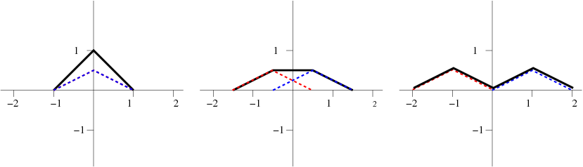
This can easily be solved graphically, as shown in Fig. 6.2.


dalembert1


Figure 6.2: The graphical form of (6.12), for (from left to right) t = 0s,t = 0.5s and t = 1s. The dashed lines are {1\over 2}f(x + t) (leftward moving wave) and {1\over 2}f(x − t) (rightward moving wave). The solid line is the sum of these two, and thus the solution u.
.

6.2.2 Finite String

The case of a finite string is more complex. There we encounter the problem that even though f and g are only known for 0 < x < a, x ± ct can take any value from −∞ to . So we have to figure out a way to continue the function beyond the length of the string. The way to do that depends on the kind of boundary conditions: Here we shall only consider a string fixed at its ends.

\begin{eqnarray} u(0,t) = u(a,t) = 0,& & %& \\ u(x,0) = f(x)\kern 2.77695pt \kern 2.77695pt {∂u\over ∂t} (x,0) = g(x).& & %&(6.13) \\ \end{eqnarray}

Initially we can follow the approach for the infinite string as sketched above, and we find that

\begin{eqnarray} F(x)& =& {1\over 2}\left [f(x) + Γ(x) + C\right ],%& \\ G(x)& =& {1\over 2}\left [f(x) − Γ(x) − C\right ].%&(6.14) \\ \end{eqnarray}

Look at the boundary condition u(0,t) = 0. It shows that

{1\over 2}[f(ct) + f(−ct)] + {1\over 2}[Γ(ct) − Γ(−ct)] = 0.
(6.15)

Now we understand that f and Γ are completely arbitrary functions – we can pick any form for the initial conditions we want. Thus the relation found above can only hold when both terms are zero

\begin{eqnarray} f(x)& =& −f(−x),%& \\ Γ(x)& =& Γ(x). %&(6.16) \\ \end{eqnarray}

Now apply the other boundary condition, and find

\begin{eqnarray} f(a + x)& =& −f(a − x),%& \\ Γ(a + x)& =& Γ(a − x). %&(6.17) \\ \end{eqnarray}


dalembert2


Figure 6.3: A schematic representation of the reflection conditions (6.16,6.17). The dashed line represents f and the dotted line Γ.

The reflection conditions for f and Γ are similar to those for sines and cosines, and as we can see from Fig. 6.3 both f and Γ have period 2a.