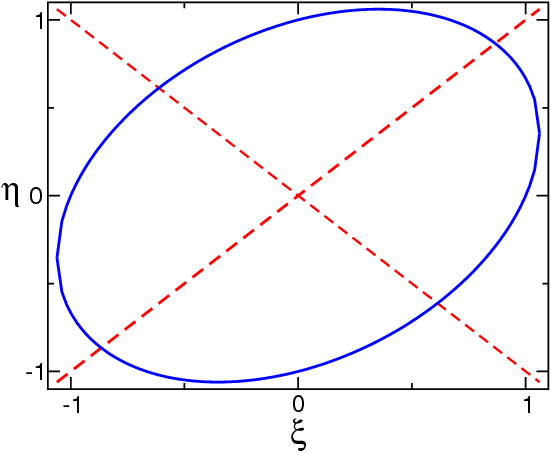
Figure 2.1: The ellipse corresponding to Eq. (2.5)
Second order P.D.E. are usually divided into three types. Let me show this for two-dimensional PDE’s:
|
a{{∂}^{2}u\over
∂{x}^{2}} + 2c {{∂}^{2}u\over
∂x∂y} + b{{∂}^{2}u\over
∂{y}^{2}} + d{∂u\over
∂x} + e{∂u\over
∂y} + fu + g = 0
| (2.2) |
where a,\mathop{\mathop{…}},g can either be constants or given functions of x,y. If g is 0 the system is called homogeneous, otherwise it is called inhomogeneous. Now the differential equation is said to be
Why do we use these names? The idea is most easily explained for a case with constant coefficients, and correspond to a classification of the associated quadratic form (replace derivative w.r.t. x and y with ξ and η)
|
a{ξ}^{2} + b{η}^{2} + 2cξη + f = 0.
| (2.4) |
We neglect d and e since they only describe a shift of the origin. Such a quadratic equation can describe any of the geometrical figures discussed above. Let me show an example, a = 3, b = 3, c = 1 and f = −3. Since ab − {c}^{2} = 8, this should describe an ellipse. We can write
|
3{ξ}^{2} + 3{η}^{2} + 2ξη = 4{({ξ + η\over
\sqrt{2}} )}^{2} + 2{({ξ − η\over
\sqrt{2}} )}^{2} = 3,
| (2.5) |
which is indeed the equation of an ellipse, with rotated axes, as can be seen in Fig. 2.1,
We should also realise that Eq. (2.5) can be written in the vector-matrix-vector form
|
(ξ,η)\left (\array{
3&1\cr
1 &3 } \right )\left (\array{
ξ\cr
η } \right ) = 3.
| (2.6) |
We now recognise that Δ is nothing more than the determinant of this matrix, and it is positive if both eigenvalues are equal, negative if they differ in sign, and zero if one of them is zero. (Note: the simplest ellipse corresponds to {x}^{2} + {y}^{2} = 1, a parabola to y = {x}^{2}, and a hyperbola to {x}^{2} − {y}^{2} = 1)