
To be used in future
Prev Section 5.1: Sum of paths
Up Chapter 5: Path Integrals
Section 5.3: Free particle revisited Next
5.2 Interpretation
After we have broken up the evolution in these small time steps, it pays to think a bit more about the interpretation of the integrals. For each value of
, we do an integration over all allowed values of
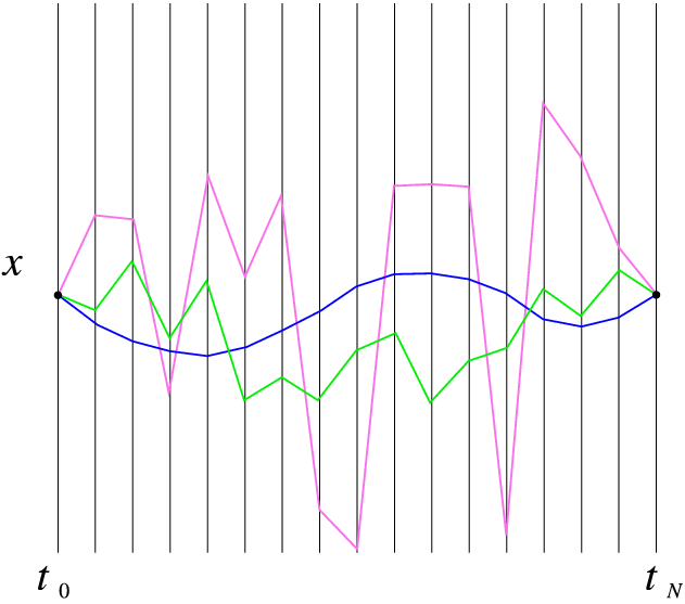
, see Fig. 5.1↓. If we think about these integrals another way, we can also argue that each possible contribution in the integral corresponds to one choice of the position
; in other words each term is a “path”
. So we can interpret the path integral as the sum over all possible paths between the two points
and
--Hence the name!
What types of paths contribute to the path integral? If we take the limiting process seriously, we get an interesting picture, see the illustrations in Fig. 5.1↑. Here the blue curve goes to a smooth path in the limit that
goes to zero, but the green and especially purple paths don’t--they seem to show some kind of almost fractal behaviour. Such fractal paths are key to the underlying Wiener process (see below). It also suggest that any path between
and
contributes, no matter how crazy--but not equally! From this simple analysis we can conclude that by construction the paths are continuous, but that they are not necessarily differentiable in the limit
. Mathematicians have studied such curves for a long time, and show that they are reasonably straightforward to deal with, so they should not be as daunting as they seem in first instance.
This work is a Open Educational Resource. Please contact Niels Walet for more information, or further licensing.
 This work is licensed under a Creative Commons Attribution-Noncommercial-Share Alike 3.0 Generic License