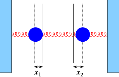
Figure 5.1: Two coupled oscillators.
In understanding the nature of a matrix (or really the linear transformation represented by it) we often would like to understand those vectors that are transformed into themselves, i.e., where
|
Ae = λe,\qquad \text{($λ$ is a constant).}
| (5.37) |
This equation is called the “eigenvalue problem”; λ is called an eigenvalue and e an eigenvector.
The question is now, obviously, how to determine λ and e. By using a simple trick, we can solve for λ without having to know e. To this end we write
|
λx = λIx = \left (\array{
λ&0\cr
0 &λ } \right )x,
|
and we can thus rewrite the eigenvalue problem as
|
(A − λI)x = 0.
| (5.38) |
We have argued in the previous section that this has only the trivial solution if \mathop{det}(A − λI)\mathrel{≠}0, i.e., x = 0. In order to avoid this we must require
|
\mathop{det}(A − λI) = 0\quad .
| (5.39) |
For a two-by-two matrix this is a simple quadratic equation.
Example 5.1:
Find the eigenvalues and eigenvectors of A = \left (\array{ 1&2\cr 2 &1} \right ).
Solution:
Solutions are λ = 1 ± 2 = −1,3.
Now determine the eigenvalues by solving (A − λI)e = 0. For {λ}_{1} = −1 we find
|
\left (\array{
2&2\cr
2 &2} \right )\left (\array{
{e}_{1}
\cr
{e}_{2}
} \right ) = 0
|
and thus {e}_{1} = −{e}_{2}, and {e}^{(1)} = c\left (\array{ 1\cr 1} \right ). The arbitrary constant can be chosen at will. Some standard choices are 1 (simple), 1∕\sqrt{2} (length 1), etc.
The same algebra for the other eigenvalue leads to {e}^{(2)} = d\left (\array{ 1\cr − 1} \right ).
If we rewrite
|
\left (\array{
x\cr
y
} \right ) = (x+y)∕2\left (\array{
1\cr
1
} \right )+(x−y)∕2\left (\array{
1\cr
− 1} \right ),
|
we can easily understand the importantce of the eigenvectors:
|
A\left (\array{
x\cr
y
} \right ) = 3(x+y)∕2\left (\array{
1\cr
1
} \right )−(x−y)∕2\left (\array{
1\cr
− 1} \right ).
|
Thus the component parallel to (1,1) is stretches by a factor of 3, and the component parallel to (−1,1) is inverted (multiplied by − 1).
The most important physical example of the role of the eigenvalue problem can be found in the case of coupled oscillators.
Consider Fig. 5.1. There we show the case of two masses, coupled by three springs. We assume that {x}_{1} and {x}_{2} are the distances of the masses from the equilibrium position. At that point we assume the strings are untentioned (neither stretched nor compressed).
The equations of motion take a simple form
We now take the masses equal ({m}_{1} = {m}_{2} = m), and all the spring constants equal as well ({k}_{1} = {k}_{2} = {k}_{3} = m{ω}^{2}. We then find that
This equation can now be solved by writing the standard exponential form, x = e{e}^{zt}. We then get
Which is an eigenvalue problem. Write {z}^{2} = {ω}^{2}λ, and we find that λ = −1,−3. Thus z = ±iω,±i\sqrt{3}ω. The eigenvectors for these two eigenvalues are (1,1) and (1,−1), respectively.
Thus, in all its generality, we find using superposition that
This general motion thus consists of the superposition of motion of the two masses in phase ({x}_{1} = {x}_{2}, with frequency ω) and one maximally out of phase ({x}_{1} = −{x}_{1}, with frequency \sqrt{3}ω).