Warning: jsMath
requires JavaScript to process the mathematics on this page.
1.5
1.5.1 We recall Euler’s formula for the sine and cosine,
\begin{eqnarray}
\mathop{exp}\nolimits (ix) =\mathop{ cos}\nolimits (x) + i\mathop{sin}\nolimits (x),& & %&(1.59) \\
\end{eqnarray}
where x is
a real number. From this, we can express sine and cosine as
\begin{eqnarray}
\mathop{cos}\nolimits (x)& :=& {1\over
2}\left ({e}^{ix} + {e}^{−ix}\right ) %&
\\
\mathop{sin}\nolimits (x)& :=& {1\over
2i}\left ({e}^{ix} − {e}^{−ix}\right ).%&(1.60) \\
\end{eqnarray}
We now define the hyperbolic functions ‘hyperbolic cosine’ and ‘hyperbolic sine’ as
\begin{eqnarray}
\mathop{cosh}\nolimits (x)& :=& {1\over
2}\left ({e}^{x} + {e}^{−x}\right ) %&
\\
\mathop{sinh}\nolimits (x)& :=& {1\over
2}\left ({e}^{x} − {e}^{−x}\right ),%&(1.61) \\
\end{eqnarray}
i.e. analogous to cosine and sine but without the imaginary unit
i . Using
{i}^{2} = −1 , we
recognise that
\begin{eqnarray}
\mathop{cosh}\nolimits (x) =\mathop{ cos}\nolimits (ix),\quad \mathop{sinh}\nolimits (x) = −i\mathop{sin}\nolimits (ix),& & %&(1.62) \\
\end{eqnarray}
which means that trigonometric and hyperbolic functions are closely related. Their behaviour as a function of
x ,
however, is different: while sine and cosine are oscillatory functions, the hyperbolic functions
\mathop{cosh}\nolimits (x) and
\mathop{sinh}\nolimits (x) are not oscillatory, because they
are just linear combinations of {e}^{x}
and {e}^{−x}
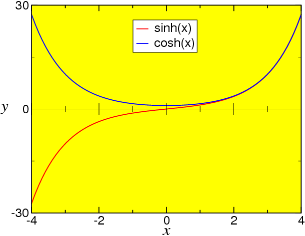
which are not oscillatory. We have the following properties:
\begin{eqnarray}
\mathop{cosh}\nolimits (0)& =& 1,\quad \mathop{cosh}\nolimits (x) =\mathop{ cosh}\nolimits (−x) %&(1.63)
\\
\mathop{cosh}\nolimits (x →∞)& →& {1\over
2}{e}^{x} {→}_{
x→∞}∞,\quad \mathop{cosh}\nolimits (x →−∞) → {1\over
2}{e}^{−x} {→}_{
x→−∞}∞ %&
\\
\mathop{sinh}\nolimits (0)& =& 0,\quad \mathop{sinh}\nolimits (x) = −\mathop{sinh}\nolimits (−x) %&
\\
\mathop{sinh}\nolimits (x →∞)& →& {1\over
2}{e}^{x} {→}_{
x→∞}∞,\quad \mathop{sinh}\nolimits (x →−∞) →−{1\over
2}{e}^{−x} {→}_{
x→−∞}−∞.%& \\
\end{eqnarray}
from which we already can sketch the two hyperbolic functions, see Fig. 1.2 .
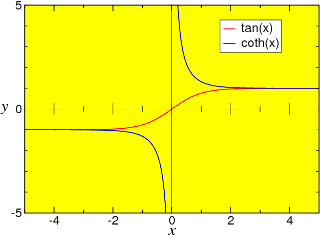
In addition, one defines the hyperbolic tangent and cotangent
\begin{eqnarray}
\mathop{tanh}\nolimits (x) := {\mathop{sinh}\nolimits (x)\over
\mathop{cosh}\nolimits (x)},\quad \mathop{coth}\nolimits (x) := {\mathop{cosh}\nolimits (x)\over
\mathop{sinh}\nolimits (x)} .& & %&(1.64) \\
\end{eqnarray}
1.5.2 Inverting
\begin{eqnarray}
y =\mathop{ sinh}\nolimits (x) → x ={\mathop{ sinh}\nolimits }^{−1}(y),& & %&(1.65) \\
\end{eqnarray}
we find the inverse hyperbolic sine {\mathop{sinh}\nolimits }^{−1}
by setting
\begin{eqnarray}
y = {{e}^{x} − {e}^{−x}\over
2} ⇝ {e}^{2x} − 2y{e}^{x} − 1 = 0.& & %&(1.66) \\
\end{eqnarray}
This is a quadratic equation in u = {e}^{x}
with the solutions
\begin{eqnarray}{
u}_{±} = y ±\sqrt{{y}^{2 } + 1}.& & %&(1.67) \\
\end{eqnarray}
Since u = {e}^{x} > 0 is positive, we must take
the positive solution {u}_{+} and must
discard the negative solution {u}_{−} .
Therefore,
\begin{eqnarray}{
e}^{x} ≡ u = y + \sqrt{{y}^{2 } + 1} ⇝ x =\mathop{ ln}\nolimits \left (y + \sqrt{{y}^{2 } + 1}\right ),& & %&(1.68) \\
\end{eqnarray}
which means that
\begin{eqnarray}
{\mathop{sinh}\nolimits }^{−1}(y) =\mathop{ ln}\nolimits \left (y + \sqrt{{y}^{2 } + 1}\right ).& & %&(1.69) \\
\end{eqnarray}
Similarly, one obtains
\begin{eqnarray}
{\mathop{tanh}\nolimits }^{−1}(y) = {1\over
2}\mathop{ln}\nolimits \left [{1 + y\over
1 − y}\right ].& & %&(1.70) \\
\end{eqnarray}
The {\mathop{cosh}\nolimits }^{−1} is a
bit more tricky.
1.5.3 These are obtained by going back to the definitions of the hyperbolic functions.
\begin{eqnarray}
\mathop{sinh}\nolimits '(x) =\mathop{ cosh}\nolimits (x),\quad \mathop{cosh}\nolimits '(x) =\mathop{ sinh}\nolimits (x),\quad \mathop{tanh}\nolimits '(x) = 1 −{\mathop{ tanh}\nolimits }^{2}(x).& & %&(1.71) \\
\end{eqnarray}
1.5.4 These also are obtained by using the definitions of \mathop{cosh}\nolimits
and \mathop{sinh}\nolimits :
\begin{eqnarray}
{\mathop{cosh}\nolimits }^{2}(x) −{\mathop{ sinh}\nolimits }^{2}(x)& =& 1,\quad \mathop{cosh}\nolimits (2x) = 1 + 2{\mathop{sinh}\nolimits }^{2}(x)%&
\\
\mathop{sinh}\nolimits (2x)& =& 2\mathop{sinh}\nolimits (x)\mathop{cosh}\nolimits (x). %&(1.72) \\
\end{eqnarray}