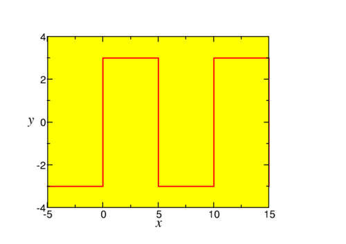
Figure 4.1: The square wave (4.23).
The series discussed before are only useful is we can associate a function with them. How can we do that?
Lets us assume that the periodic function f(x) has a Fourier series representation (exchange the summation and integration, and use orthogonality),
|
f(x) = {{a}_{0}\over
2} +{ \mathop{∑
}}_{n=1}^{∞}\left [{a}_{
n}\mathop{ cos}\nolimits \left ({nπx\over
L} \right ) + {b}_{n}\mathop{ sin}\nolimits \left ({nπx\over
L} \right )\right ].
| (4.18) |
We can now use the orthogonality of the trigonometric functions to find that
This defines the Fourier coefficients for a given f(x). If these coefficients all exist we have defined a Fourier series, about whose convergence we shall talk in a later lecture.
An important property of Fourier series is given in Parseval’s lemma:
|
{\mathop{\mathop{\mathop{∫
}\nolimits }}\nolimits }_{−L}^{L}f{(x)}^{2}dx = {L{a}_{0}^{2}\over
2} + L{\mathop{∑
}}_{n=1}^{∞}({a}_{
n}^{2} + {b}_{
n}^{2}).
| (4.22) |
This looks like a triviality, until one realises what we have done: we have once again interchanged an infinite summation and an integration. There are many cases where such an interchange fails, and actually it make a strong statement about the orthogonal set when it holds. This property is usually referred to as completeness. We shall only discuss complete sets in these lectures.
Now let us study an example. We consider a square wave (this example will return a few times)
|
f(x) = \left \{\array{
−3\quad &\text{ if $ − 5 + 10n < x < 10n$}\cr
3 \quad &\text{ if $10n < x < 5 + 10n$} } \right .\quad ,
| (4.23) |
where n is an integer, as sketched in Fig. 4.1.
This function is not defined at x = 5n. We easily see that L = 5. The Fourier coefficients are
And thus (n = 2m + 1)
|
f(x) = {12\over
π} {\mathop{∑
}}_{m=0} {1\over
2m + 1}\mathop{sin}\nolimits \left ({(2m + 1)πx\over
5} \right ).
| (4.25) |
Question: What happens if we apply Parseval’s theorem to this series?
Answer: We find
|
{\mathop{\mathop{\mathop{∫
}\nolimits }}\nolimits }_{−5}^{5}9dx = 5{144\over
{π}^{2}} { \mathop{∑
}}_{m=0}^{∞}{\left ( {1\over
2m + 1}\right )}^{2}
| (4.26) |
Which can be used to show that
|
{\mathop{∑
}}_{m=0}^{∞}{\left ( {1\over
2m + 1}\right )}^{2} = {{π}^{2}\over
8} .
| (4.27) |