10.8 Fourier-Bessel series

So how can we determine in general the coefficients in the Fourier-Bessel series

f(ρ) ={ \mathop{∑ }}_{j=1}^{∞}{C}_{ j}{J}_{ν}({α}_{j}ρ)?
(10.71)

The corresponding self-adjoint version of Bessel’s equation is easily found to be (with {R}_{j}(ρ) = {J}_{ν}({α}_{j}ρ))

(ρ{R}_{j}')' + ({α}_{j}^{2}ρ −{{ν}^{2}\over ρ} ){R}_{j} = 0.
(10.72)

Where we assume that f and R satisfy the boundary condition

\begin{eqnarray} {b}_{1}f(c) + {b}_{2}f'(c)& =& 0%& \\ {b}_{1}{R}_{j}(c) + {b}_{2}{R}_{j}'(c)& =& 0%&(10.73) \\ \end{eqnarray}

From Sturm-Liouville theory we do know that

{\mathop{\mathop{\mathop{∫ }\nolimits }}\nolimits }_{0}^{c}ρ{J}_{ ν}({α}_{i}ρ){J}_{ν}({α}_{j}ρ) = 0\kern 2.77695pt \kern 2.77695pt if\ i\mathrel{≠}j,
(10.74)

but we shall also need the values when i = j!

Let us use the self-adjoint form of the equation, and multiply with 2ρR', and integrate over ρ from 0 to c,

{\mathop{\mathop{\mathop{∫ }\nolimits }}\nolimits }_{0}^{c}\left [(ρ{R}_{ j}')' + ({α}_{j}^{2}ρ −{{ν}^{2}\over ρ} ){R}_{j}\right ]2ρ{R}_{j}'dρ = 0.
(10.75)

This can be brought to the form (integrate the first term by parts, bring the other two terms to the right-hand side)

\begin{eqnarray} {\mathop{\mathop{\mathop{∫ }\nolimits }}\nolimits }_{0}^{c} {d\over dρ}{\left (ρ{R}_{j}'\right )}^{2}dρ& =& 2{ν}^{2}{\mathop{ \mathop{\mathop{∫ }\nolimits }}\nolimits }_{0}^{c}{R}_{ j}{R}_{j}'dρ − 2{α}_{j}^{2}{\mathop{ \mathop{\mathop{∫ }\nolimits }}\nolimits }_{0}^{c}{ρ}^{2}{R}_{ j}{R}_{j}'dρ%&(10.76) \\ { \left .{\left (ρ{R}_{j}'\right )}^{2}\right |}_{ 0}^{c}& =&{ \left .{ν}^{2}{R}_{ j}^{2}\right |}_{ 0}^{c} − 2{α}_{ j}^{2}{\mathop{ \mathop{\mathop{∫ }\nolimits }}\nolimits }_{0}^{c}{ρ}^{2}{R}_{ j}{R}_{j}'dρ. %&(10.77) \\ \end{eqnarray}

The last integral can now be done by parts:

\begin{eqnarray} 2{\mathop{\mathop{\mathop{∫ }\nolimits }}\nolimits }_{0}^{c}{ρ}^{2}{R}_{ j}{R}_{j}'dρ& =& −2{\mathop{\mathop{\mathop{∫ }\nolimits }}\nolimits }_{0}^{c}ρ{R}_{ j}^{2}dρ +{ \left .ρ{R}_{ j}^{2}\right |}_{ 0}^{c}.%&(10.78) \\ \end{eqnarray}

So we finally conclude that

2{α}_{j}^{2}{\mathop{ \mathop{\mathop{∫ }\nolimits }}\nolimits }_{0}^{c}ρ{R}_{ j}^{2}dρ ={ \left [\left ({α}_{ j}^{2}{ρ}^{2} − {ν}^{2}\right ){R}_{ j}^{2} +{ \left (ρ{R}_{ j}'\right )}^{2}\right |}_{ 0}^{c}.
(10.79)

In order to make life not too complicated we shall only look at boundary conditions where f(c) = R(c) = 0. The other cases (mixed or purely f'(c) = 0) go very similar! Using the fact that {R}_{j}(r) = {J}_{ν}({α}_{j}ρ), we find

{R'}_{j} = {α}_{j}{J'}_{ν}({α}_{j}ρ).
(10.80)

We conclude that

\begin{eqnarray} 2{α}_{j}^{2}{\mathop{ \mathop{\mathop{∫ }\nolimits }}\nolimits }_{0}^{c}{ρ}^{2}{R}_{ j}^{2}dρ& =&{ \left [{\left (ρ{α}_{ j}{J'}_{ν}({α}_{j}ρ)\right )}^{2}\right |}_{ 0}^{c} %& \\ & =& {c}^{2}{α}_{ j}^{2}{\left ({J'}_{ ν}({α}_{j}c)\right )}^{2} %& \\ & =& {c}^{2}{α}_{ j}^{2}{\left ( {ν\over { α}_{j}c}{J}_{ν}({α}_{j}c) − {J}_{ν+1}({α}_{j}c)\right )}^{2}%& \\ & =& {c}^{2}{α}_{ j}^{2}{\left ({J}_{ ν+1}({α}_{j}c)\right )}^{2}, %&(10.81) \\ \end{eqnarray}

We thus finally have the result

{\mathop{\mathop{\mathop{∫ }\nolimits }}\nolimits }_{0}^{c}{ρ}^{2}{R}_{ j}^{2}dρ = {{c}^{2}\over 2} {J}_{ν+1}^{2}({α}_{ j}c).
(10.82)

Example 10.1: 

Consider the function

f(x) = \left \{\array{ {x}^{3}&\kern 2.77695pt \kern 2.77695pt 0 < x < 10 \cr 0 &\kern 2.77695pt \kern 2.77695pt x > 10} \right .
(10.83)

Expand this function in a Fourier-Bessel series using {J}_{3}.

Solution: 

From our definitions we find that

f(x) ={ \mathop{∑ }}_{j=1}^{∞}{A}_{ j}{J}_{3}({α}_{j}x),
(10.84)

with

\begin{eqnarray}{ A}_{j}& =& {2\over 100{J}_{4}{(10{α}_{j})}^{2}}{\mathop{ \mathop{\mathop{∫ }\nolimits }}\nolimits }_{0}^{10}{x}^{3}{J}_{ 3}({α}_{j}x)dx %& \\ & =& {2\over 100{J}_{4}{(10{α}_{j})}^{2}} {1\over { α}_{j}^{5}}{\mathop{ \mathop{\mathop{∫ }\nolimits }}\nolimits }_{0}^{10{α}_{j} }{s}^{4}{J}_{ 3}(s)ds %& \\ & =& {2\over 100{J}_{4}{(10{α}_{j})}^{2}} {1\over { α}_{j}^{5}}{(10{α}_{j})}^{4}{J}_{ 4}(10{α}_{j})ds%& \\ & =& {200\over { α}_{j}{J}_{4}(10{α}_{j})}. %&(10.85) \\ \end{eqnarray}

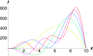
Using {α}_{j} = \mathop{\mathop{…}}, we find that the first five values of {A}_{j} are 1050.95,−821.503,703.991,−627.577,572.301. The first five partial sums are plotted in Fig. 10.6.


Besselx3


Figure 10.6: A graph of the first five partial sums for {x}^{3} expressed in {J}_{3}.