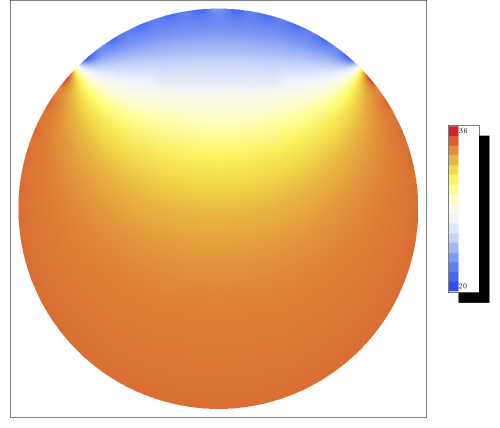
Let me return to my model of the eye. With the functions {P}_{n}(\mathop{cos}\nolimits θ) as the solution to the angular equation, we find that the solutions to the radial equation are
|
R = A{r}^{n} + B{r}^{−n−1}.
| (11.36) |
The singular part is not acceptable, so once again we find that the solution takes the form
|
u(r,θ) ={ \mathop{∑
}}_{n=0}^{∞}{A}_{
n}{r}^{n}{P}_{
n}(\mathop{cos}\nolimits θ)
| (11.37) |
We now need to impose the boundary condition that the temperature is 2{0}^{∘} C in an opening angle of 4{5}^{∘}, and 3{6}^{∘} elsewhere. This leads to the equation
This leads to the integral, after once again changing to x =\mathop{ cos}\nolimits θ,
These integrals can easily be evaluated, and a sketch for the temperature can be found in figure 11.3.

Notice that we need to integrate over x =\mathop{ cos}\nolimits θ to obtain the coefficients {A}_{n}. The integration over θ in spherical coordinates is {\mathop{\mathop{\mathop{∫ }\nolimits }}\nolimits }_{0}^{π}\mathop{ sin}\nolimits θdθ ={\mathop{ \mathop{\mathop{∫ }\nolimits }}\nolimits }_{−1}^{1}1dx, and so automatically implies that \mathop{cos}\nolimits θ is the right variable to use, as also follows from the orthogonality of {P}_{n}(x).