
To be used in future
Prev Section 6.4: Graphene
Up Chapter 6: Relativistic wave equations
Appendix A: Useful Mathematics Next
6.5 Spherical symmetry↓
We often look at potentials with spherical symmetry, usually because the (sub-)atomic world is rotationally invariant—there are no preferred directions.
We consider the simplest case of a particle confined to a potential well that couples like the zeroth component of four-vector; the other option (where we see a scalar potential and effectively the mass becomes position dependent can be dealt with in exactly the same way)
we now look at the symmetries of
. Clearly, the angular momentum operator
acts nontrivially on
and thus
Fortunately the commutator with
is minus this result
and thus
commutes with
. [O] [O] Once again we have been slightly careless: we should say that
is a matrix of operators, with
. We also need the analogue of space inversion symmetry; the standard inversion operator
, which acts on functions of
,
must of course be used, but we also need to add a matrix part since the symmetry is allowed to act on each component differently. Since the momentum operator
is odd under parity,
the matrix part of the operation must leave
and
invariant, but change the sign of
. It is easy to find that the matrix
has these properties, and we shall thus define the parity operator as
since
From the standard form
we see that the lower components of
are multiplied with an additional minus sign under a parity transformation, independent of the parity of the function in these components. This additional minus sign is used to state that these components have negative “intrinsic parity”, something you may pick up in your particle physics course as well!
We shall now try to resolve the solutions to the Dirac equation in states that are both parity and angular momentum eigenstates. We first decompose in upper and lower components,
where we impose parity,
6.5.1 Role of vector spherical harmonics
It is reasonably hard work to find states of good angular momentum, but we do know the solution: combine the eigenstates of
(spherical harmonics) with the spinors describing spin-
states into so-called vector spherical harmonics (the parity quantum number
)
Here
is completely determined by the parity
, which we know equals
. It is slightly more efficient to replace parity for a state of angular momentum
by another quantum number,
which has the additional advantages that we can capture the Clebsch-Gordan coefficients above in the very compact form,
and include some of the information about
, since we find
We can now finally write the wave function as (the
in the lower components is conventional, and will simplify later calculations)
This satisfies
We need to evaluate the action of
on a vector-spherical harmonic. Start with the identity
Thus we can write
The attraction of this expression is that anything involving
or
only acts on the angular components of the wave function, and we shall show below that
The first step in proving these relations is to show that
so that neither operator can change the
values. In the first case (↓) we see that since
has negative parity, we must have
on the right-hand side. Using [P] [P] As usual, we write
.
we see that the magnitude in Eq. (↓) is correct--the phase is purely a matter of an arbitrary choice of phase in the definition of
for different
. The choice made here is the most common one.
This standard choice corresponds to the Condon and Shortley phase as discussed in Judith McGovern's notes , or mathworld http://mathworld.wolfram.com/Condon-ShortleyPhase.html
The second relation (↓) is an eigenvalue equation. It is most easily solved by writing
6.5.2 Radial equations
We now get the coupled equations
or cancelling the common vector-spherical harmonics,
If we make the usual substitution for the radial functions,
and
, [Q] [Q] To confuse matters, some textbooks use
for upper and
for the lower component! we get the standard result
6.5.3 Hydrogen-like atom
6.5.3.1 Relativistic approach
We start from Eqs. (↓), and use the Coulomb potential
It helps to change units to suit the problem: with
we get
We now seek solutions of the form of an exponential times a finite polynomial (the fact that the sums for
and
end at the same
is something we can show by performing more analysis)
We get the recurrence relation
For
we find
Thus
If we wish the wavefunction to behave nicely at the origin (integrable singularity), we must have
. Need to take positive square root! [R] [R] For
, the smallest
can be is
, as long as
.
Now use
to derive from
in Eqs. (↓) that
Now look at
, and eliminate the
coefficients
We now use the value of
,
,
:
and solve for
,
This impressive expression can be Taylor expanded in powers of
; most conveniently define the “normal” principal quantum number, i.e., the equivalent of the one used in non-relativistic quantum mechanics,
to find that
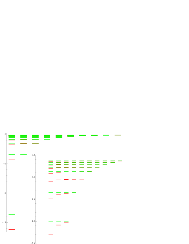
This clearly shows that the degeneracy (in
) for the non-relativistic hydrogen atom is broken by the next-to-leading order term. These corrections are actually quite small for Hydrogen, but not for
, see Fig. 6.8↓.
It is finally instructive to look at the relativistic ground state wave function
For
close to 1 we clearly have a very different behaviour near the origin. We can see this in the probability distributions as shown in Fig. 6.9↓, where the probability of the lower component increases dramatically as
increases, peaking closer and closer to zero.
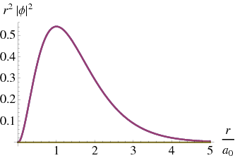
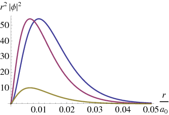
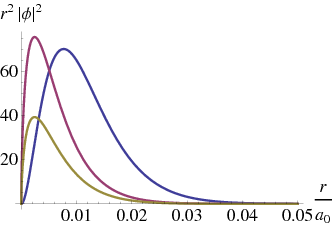
Figure 6.9 The ground state wave function for the Hydrogen wave function, for three values of
: from left to right
,
,
. In each case the blue curve is the nonrelativistic result; the red curve is the contribution of the upper component of the relativistic result, and the gold curve shows the lower component.
This work is a Open Educational Resource. Please contact Niels Walet for more information, or further licensing.
 This work is licensed under a Creative Commons Attribution-Noncommercial-Share Alike 3.0 Generic License