
To be used in future
Prev Section 6.3: Dirac equation
Up Chapter 6: Relativistic wave equations
Section 6.5: Spherical symmetry Next
6.4 Graphene↓
A prime example of a non-fundamental system that can be described by a Dirac equation is graphene. A material important enough to give the Nobel price in 2010 to Andrei Geim and Kostya Novoselov. Let me explain the basics.
6.4.1 Tight binding model
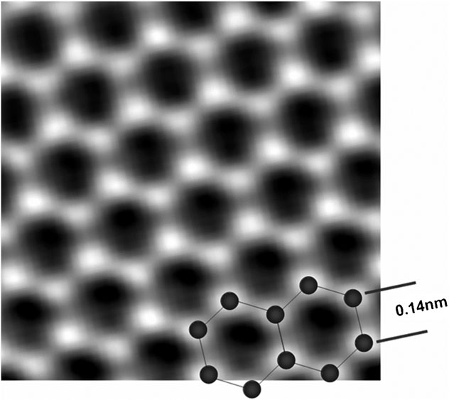
Graphene is the technical term used for a structure made of one (sometimes a few) layer of a two-dimensional sheet of carbon, see Fig. 6.3↑ for a sketch and TEM image.
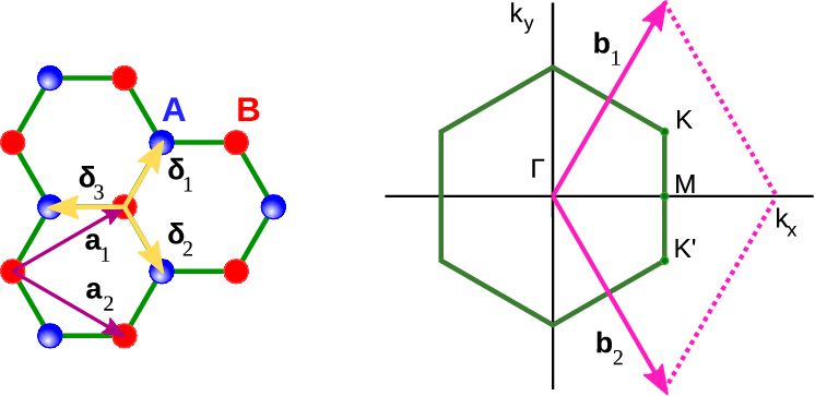
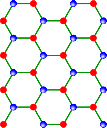
There is a very natural way to describe the lattice; as we can see in Fig. 6.4↑ we have two natural sublattices; the lattice vectors
connect all states in one sublattice )(which is triangular). The reciprocal lattice vectors have the form
Each point in one sublattice is linked by three “nearest-neighbour vectors” to the other sublattice,
The simplest way to model a system like graphene, is to model the overlap of free electrons--in an almost chemical way. The underlying technique is called the tight binding (LCAO) method [14]. [M] [M] First applied to graphite (and graphene) by Wallace in 1947 (Phys. Rev. 71, 622) We assume that an individual electron lives in a superposition of the same orbits over all the atomic sites
where
sums over all the atoms, but
can only depend on an index that labels atoms that are inequivalent under lattice symmetries (translation/rotation). For the case of graphene, we can split the normal lattice into two inequivalent sublattices
and
, see Fig. 6.4↑, corresponding to the two atoms in a primitive unit cell. The energy expectation value for states with momentum
is then, in the tight-binding approximation,
where
is the sublattice sum, and here
enumerates the atoms of type
that couple to
.
We assume only nearest neighbour coupling. Each atom has three nearest neighbours a distance
away which all lie on the “other” sublattice, but otherwise equivalent, and thus
We now minimise the energy w.r.t. the coefficients
, and get an effective two-by-two Hamiltonian for the determination of the coefficients
,
where
and
labels the three nearest neighbours. Since the diagonals are equal, we may as well choose them
, setting the zero of energy,
Since all the three neighbour sites are completely equivalent, the coupling (tight-binding) between the point we are interested in and the neighbours is ruled by one parameter which is usually called
,
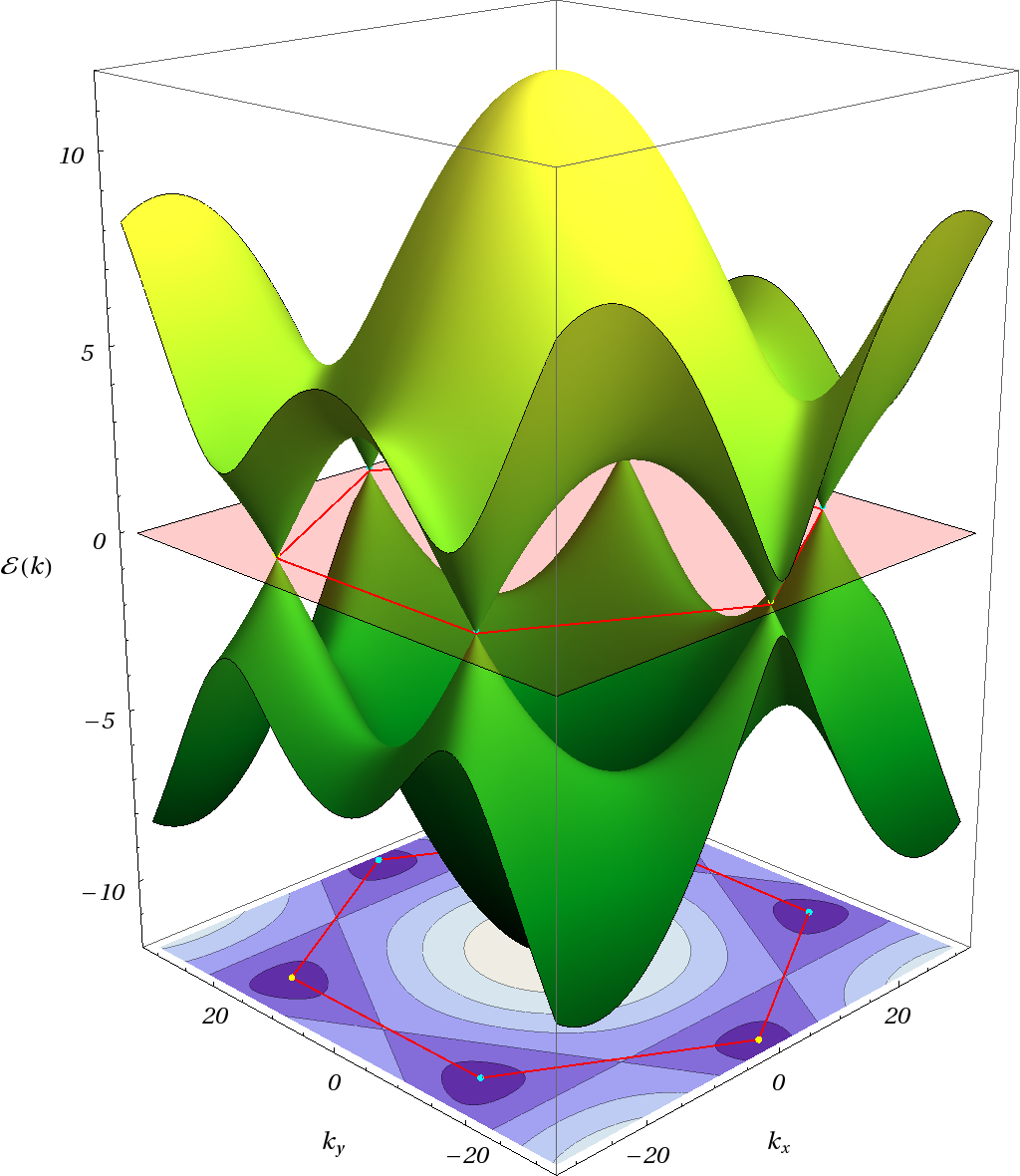
We can now find the two eigenenergies of the matrix (↓) as a function of
,
These energies are show as a function of
in Fig. 6.5↓.
6.4.2 Dirac points--Dirac equation
Since the normal number of electrons is such that the energy states are half-filled, all states in the lower surface are filled. Something strange happens in the vicinity of the point where the energy is degenerate (see Fig. 6.5↑). It takes no energy at all to hop between the surfaces at the point; thus the states nearby describe the low-energy excitations, the dynamics of electrons and holes. The easiest way to find how this happens is to solve for
, i.e., the tight-binding Hamiltonian is diagonal. A little thought shows that at that point
must be real, and we easily identify the six solutions:
Of these six, there are only two inequivalent ones (others can be reached by the reciprocal lattice vectors
). Any two adjacent points on the hexagon can be used; we choose
.
It is interesting to look at the behaviour of the interaction near those points; write
with
small. We find
We get two two-by-two Hamiltonians of the form
Combining the two corresponding wave functions
(each length 2) at a single energy into a single length 4 vector, rotating
and using
we get the equation
which is the Dirac equation for massless particles in 2 dimensions, once we replace
by the Fermi velocity
.
Since the particles are massless, the logical basis to use is the helicity basis discussed above.
6.4.3 Klein paradox and graphene
Since it is described by a massless Dirac equation, the question about the behaviour under scattering has been asked.
6.4.3.1 Simple potential barrier
The easiest thing to do is to consider a simple potential barrier of height
and width
. Using the matching technique used above we can show that for a wave impinging in the perpendicular direction on the barrier the coefficient of the reflected and transmitted wave function is
where
We can thus either have
both real or both purely imaginary. In both cases
. We see that the transmission goes to 1 as the mass goes to zero, as we expect in graphene.
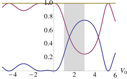
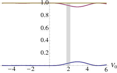
Figure 6.6 The tunnelling and reflection probability for a Dirac particle impinging on a barrier of height
. The energy is
, and
is 1 on the left and
on the right (all expressed in the same arbitrary units). The red line shows the transmission, the blue line the reflection. The grey energy band is where the momentum inside the barrier is imaginary.
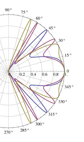
6.4.3.2 Picture of general result
In general we can also have scattering under an oblique angle; this has been evaluated in the literature [N] [N] Katsnelson, Geim, Novoselov (see also example sheet). For a massless particle we get the picture
6.4.3.3 Experimental data↓
This work is a Open Educational Resource. Please contact Niels Walet for more information, or further licensing.
 This work is licensed under a Creative Commons Attribution-Noncommercial-Share Alike 3.0 Generic License