
To be used in future
Prev Section 6.2: Klein-Gordon equation
Up Chapter 6: Relativistic wave equations
Section 6.4: Graphene Next
6.3 ↓Dirac equation
The Schrödinger equation is first order in time, whereas the Klein-Gordon equation contains a double derivative. We know that if we Taylor-expand the square root that describes energy, we can find the non-relativistic energy. Should we have worked with the square-root instead? If we wish to avoid the problems with negative probability and negative energy solutions, we can try to find an alternative wave equation. Since it has to be first order in time derivatives, we must deal with the square-root problem head on. We shall sketch two methods to derive such an equation.
6.3.1 Using minimal coupling
Let me reind you of the discussion of the Pauli-Schrödinger equation given in Sec. 4.7↑. There we found that the Schrödinger equation for a particle with spin (coupled to an electro-magnetic field can be given by the Pauli-Schrödinger equation
We shall now try and find the relativistic analogue of this equation.
6.3.1.1 Relativistic form
We now look again at the relativistic energy-momentum relationship,
and deal with that using similar techniques. We write an operatorial equation, using the correspondence principle,
We use the normal definition of the energy operator as a time derivative,
We thus get the wave equation
where
is a two-component wave function. We can get an equation linear in time-derivatives—and by Lorentz symmetry momentum— by doubling up on the components,
and find
defining
we get
which leads to the standard covariant form of the Dirac equation,↓
with
The usual derivation, as given below, results in an equivalent form which is closer to the normal Schrödinger equation, which we can obtain by multiplying our result (↓) by
from the left↓
where we have defined
We now identify the Hamiltonian operator with the left-hand side since the right-hand side is clearly the energy operator,↓
A possible explicit form of the matrices
and
are given below (↓), and in more detail, with the four
matrices, in appendix A.9↓.
6.3.2 The Classical solution: Linearisation of the energy momentum relationship
Dirac came up with the idea to linearise the energy momentum relationship, i.e., write
with the requirement on the square that
It is immediately clear that
and
can not be numbers. If we calculate
assuming order of multiplcation matters, we find they must satisfy
Dirac’s idea was to solve this with matrices; the lowest dimension where we can find four such matrices is 4; there are many solutions that can all be shown to be equivalent [A] [A] I.e., they can be written in the form
and
with a single unitary matrix transformation
., and we shall use the canonical choice (see appendix for full expressions)
So
is interpreted as the matrix sum
Dirac postulated the following wave equation, using the correspondence principle to replace
by the canonical operator
, and realising that the energy operator is the generator of evolution,
We see that in this equation
must be a four-component vector of functions, since the operator on the left-hand side is a four-by-four matrix of operators.
6.3.3 Plane wave solutions↓
So what are the solutions to (↓) for a free particle? We once again try a plane wave, or more precisely, a length four vector
times a single common exponential factor,
and find, writing the length four vector
in terms of two length two vectors
and
, usually called the upper and lower components of the wave function, respectively,↓↓↓
that
These are relatively straightforward coupled equations
We can eliminating
in favour of
using Eq. (↓),
and thus find
If we substitute use the expression (↓) for
in (↓), and multiply both sides of the equation by
we get the equation
Thus
and we clearly not resolved the negative energy problem--negative
’s are still allowed. We should not be surprised, because this seems inherently linked to relativity--the energy momentum relation has this structure, and will always allow for negative energy solutions, unless we give up on the correspondence principle.
6.3.3.1 Positive energy solutions↓
We normally look for positive energy solutions of the form
where
for quantisation along the
-axis.
Proof of correctness (for
;
follows the same roue)
These are conventionally normalised to
, [B] [B] As per usual, there are many other conventions in the literature; the most common alternative is
. which gives
6.3.3.2 Negative energy solutions↓
For negative energy we find the form (using the technique shown above)
again normalised to
. For subtle reasons we choose
6.3.3.3 Spin?
This choice of
and
is not unique; but has the advantage that they becomes very simple as
(as long as the particle has a non-zero rest mass):
These are all eigenstates of the third component of the “spin operator”
It is at this point we identify them as particles with spin up (1 and 4) or down (2 and 3).
6.3.3.4 Zero rest mass: helicity basis↓
As said before, these are not the optimal choice for massless particles. A simple calculation show that the standard basis takes the form
The result would be simpler if we use the eigenvectors of
, the spin in the direction of motion (the spin is either parallel or antiparallel, corresponding to the spin projection
) as our basis:
With this choice we can define a new and very elegant basis,
This is called the helicity (handedness) basis; we call a fermion left-handed if the spin projection is parallel to the momentum, and right-handed if it is antiparallel. Since we can never overtake a relativistic massless particle, the helicity eiegnvalue is Lorentz invariant, and this is thus a Lorentz invariant choice!
6.3.3.5 Charge conjugation
One of the manipulations that leaves the Dirac equation invariant is “charge conjugation↓”, a process that turns a positive energy state in a negative one. We shall show that this corresponds to a symmetry transformation of the form
with
Invariance of the Dirac equation states that both
and
must satisfy the same Dirac equation. To show this we start from
Taking the complex conjugate we find that
where the minus sign arises since
(i.e., we are only taking complex conjugates--not a Hermitean conjugate). We further find from the explicit form of the
’s that
Thus
and we find that
as required. The transformation (↓) clearly turns a solution into another solution.
So why do we call the symmetry charge conjugation? This terminology arises when we look at the coupling to electromagnetic fields. For simplicity we only consider a vector potential,
On charge conjugation,
changes sign, but since it is real
does not, so
and we have obtained an equation for what is clearly a particle of opposite charge.
The picture becomes more elegant if we look at what the symmetry does to the plane wave solutions. Look at a positive energy solution
where we have
clearly a plane wave of negative energy, and opposite momentum. So let us look at the 4-spinor multiplying this
Thus our basic basis is charge-conjugation symmetric. [C] [C] Actually, we also see why
was defined in the opposite order with a minus sign as compared to
; this removes any phase factors.
6.3.3.6 Completeness↓↓
We can decompose any vector in
’s and
’s. Please try to prove that
and explain the relevance of this result.
6.3.4 Probability
So can we write a continuity equation with a positive probability? It could well work, and a natural assumption for the probability density is
We use
where the left-pointing arrow shows that the derivative acts to the left, to find
We thus identify
Since
, the Dirac equation can be given a probabilistic interpretation in the classical sense.
6.3.5 Klein Paradox↓
Suppose we are looking at several regions of constant but different potential energy
; assume a coupling as a vector potential (component of a four-vector). We simply modify the Dirac equation in each region to become
Let us consider two region separated by a plane: Assume that for
,
, and for
,
>0. Consider a plane wave that comes in along the
-axis, from the negative
direction, with momentum
and polarisation
,
where we impose a positive energy solution
and use
Here we can and shall ignore any normalisation factor, which is linked to a normalisation of total flux—we are interested in relative behaviour, not absolute values!
The reflected wave can have both polarisations,
and the transmitted wave as well
with
Since the Dirac equation contains only first order derivatives, it is clear that the boundary condition is that all four components of the wave function are continuous,
Since the
’s are length four vectors, these are four equations with four unknowns; looking at the 2nd and 4th equation, we find polarisation is preserved,
. Solving for the remaining coefficients we have
We easily derive
with
In order to calculate the reflection and transmission coefficients, we must calculate the probability currents, which only flow in the
direction
(we make the assumption that we have chosen the energy such that only
is potentially complex). We find that the reflection of transmission coefficients as the ratios of the currents,
We can show that
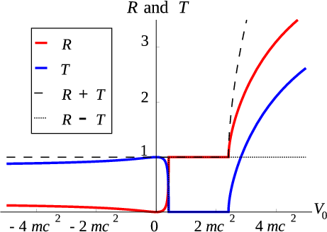
as expected. If we naively calculate the coefficients for all values of
, we find the results shown in Fig. 6.2↓. We notice that we always get some reflection when the barrier rises above the kinetic energy, reflection goes to one and transmission to zero. Below this we see standard picture, where there is some sensitivity to the depth of the potential. As we increase the barrier height beyond
, we get an enormous increase in both reflection and transmission--it almost looks like we are creating probability. This is called Klein’s paradox. [D] [D] Even though Oscar Klein originally proved this for the Dirac equation, the Klein-Gordon equation suffers from the same defect.
If we evaluate
we indeed find a real solution--but are we missing the fact that we have a negative energy solution on the right of the barrier? We can show that
which is the negative energy spinor—so we can take energy negative without fear, apart from a required flip in momentum. This interpretation is interesting since it requires that we must assume that the phase velocity (
) changes sign, but the group velocity
does not. Even these days this issue is still being argued about [E] [E] See D. Dragoman, Phys. Scr. 79 (2009) 015003, doi:10.1088/0031-8949/79/01/015003. The fact that the current flows to the left even in the right-hand side area, suggests that with a sensible interpretation [F] [F] See the Quantum Field Theory course in Year 4, where all the negative energy states are occupied, we have a hole (antiparticle) moving in the opposite direction to the particle. As we increase the barrier, the allowed negative energy solutions on the right align with an incoming positive energy wave, so we expect the transmitted wave to be present again. What we do not expect is the increase in (initially transmission but later also reflection) probability beyond 1. If we look at the difference between reflected and transmitted current, we note that we seem to have full penetration of the current to the right, but an additional pair of equal but opposite currents is added on top of this effect. What we see is in effect a signature of the creation of particle-antiparticle pairs from the vacuum. You may want to look up the discussion of this phenomenon in a textbook!
What this means, is that we interpret the negative energy states as a reservoir of fully filled states—called the Dirac sea—so that we need to work in a new framework, where we can promote a particle from the occupied Dirac sea to the empty positive energy states. If we interpret the hole in the sea (which has opposite charge to the to the original particles) as an antiparticle, we see that there is a pair creation process possible, where we create a particle-antiparticle pair. In the case discussed above, the incoming particle can create such a pair, so that we can have two particles and one-antiparticle emerge, while only a single particle comes in. This is the standard interpretation of Klein’s paradox.
This effect is of course much more prominent for massless particles: for the fermionic analogue of the photon—e.g., a massless neutrino, we find
where we have
and thus the currents diverge.
If we have a small barrier of width
and height
we can show that no such problems occur. This is discussed in a problem on the example sheet and below for graphene.↓
6.3.6 Lorentz transformations and external field
We still need to understand how the Dirac equation behaves under Lorentz transformation. The “covariant form” of the equation is most useful here,↓
This is often written in the “Feynman slash” notation
which
.
6.3.6.1 Coupling to external fields
One we have a covariuant form, we can understand how to couple to extrenal fields. We get two classes:
- Scalar fields, which are the same in every Lorentz frame. This is analogous to the rest mass, which is frame independent, i.e., a scalar field enters with the rest mass term.
- Vector fields, which behave like a four-vector. A prime example is the electromagnetic field , or with the coupling parameters . This must enter through minimal coupling.
This leads to the equation
and in non-covariant form we get
6.3.6.2 Lorentz covariance
If it is to make sense, the same form of Dirac equation must be satisfied in the new coordinate system
, where (see section A.6↓ for details of the notation, but succinctly this states that the derivatives transform under the inverse Lorentz transformation)
And thus
Let us assume that the relation between
and
’ is linear, [G] [G] We are guided by the behaviour of the non-relativistic case that this transformation is realised in a linear manner.
If we further impose that we choose the same form for the
matrices in both frames of reference [H] [H] That is not a requirement; we can accept changes to
as well, but it leads to unnecessary additional complications.,
, we find that we can rewrite (↓) after multiplication with
from the left as
This must be the original Dirac equation, and thus we must impose
which can be rewritten as [I] [I] This is the active formulation;
transforms
to
. Many books use the equivalent result for a passive transformation. This is identical, but gives a number of minus signs in the derivation below. (As an example see Ref.\ [7].)
Actually it is easiest to look at an infinitesimal transformation first, see Eq. (↓). We call the small correction to the unit transformation
and write
Raising and lowering indices to get the inverse of
we get to lowest order in
,
and thus
Multiplying by
we can raise the lower indices on both
’s
and we find
Thus
is antisymmetric, and we find that we have only six independent parameters we need to fix to specify it (the number of independent entries in an antisymmetric
matrix).
Let us look at two examples:
-
In this case we have . Using we get , and the matrix is symmetric A simple calculation shows that and we have a boost along the -axis. -
In this case we have . Using we get , and the matrix is anti-symmetric: A simple calculation shows that and we have a rotation along the -axis.
The parameters
specify the infenitessimal Lorentz transformation; they must also appear in
on the left-hand side, because
will clearly depend on the specific Lorentz transformation being made. Thus we can expand
in these quantities as well. Since there are no free indices on
, it must be multiplied by a set of matrices with the same indices. Those matrices better be independent of
! Once again, we only need consider a constant plus a linear term, which we choose in the suggestive form [J] [J] The factor
is for ease of calculation.
where the
are a set of as yet unknown
matrices (i.e., for each
we have a different matrix, c.f. the
matrices). We now substitute Eq. (↓) into Eq. (↓), and concentrate on the terms linear in
:
Here we have used the antisymmetry of
to get be able to subtract to equivalent terms, and changed the dummys summation indix in one of the terms. Thus
From this it is easy to show that
Check:
Using the relation (↓).
Thus we find that the matrices
indeed do not depend on the Lorentz transformation.
6.3.6.3 Finite transformations
If we wish to calculate finite transformations, we find trivially
a nice expresion, but not so easy to interpret. It helps if we distinguish between boosts and rotations (and by multiplication, we can then work out what happens in general).
The most general rotation can be written as a combination of boost and rotations. In the case of a rotation parametrised in the “unwise” way
with [K] [K] As you can check,
In terms of the
’s, we have siz non-zero entries in the matrix
We need to work out (note the lowered index on
, that give rise to additional minus signs)
Thus we find that
where the facor
has disappeared since we have two contributions for each
, see Eq. (↓). This confirms the identification of
with the angular momentum operator,.
For a pure boost, we have
with [L] [L] As you can check,
, which is one of the reasons for complications, and not considering the full set of transformationa as a whole.
or, in other words,
Since
we find that
Whereas in the case of rotations
is unitary, in general it is not. Fortunately, we can show a relation between the inverse and the hermitean conjugate is simple:
We can show that the matrix
satisfies the useful relation
Please try to prove this yourself.
6.3.7 Non-relativistic limit
The non-relativistic limit is obtained for small momenta, mathematically this means we expand in powers of the dimensionless quantity
; this is most easily demonstrated for a free particle. If we start with the positive energy states. we find that
and for negative energy we get the form
6.3.8 Zitterbewegung
For this section we choose to work in the Heisenberg representation, where the wave function is time independent, but the time-evolution is carried by the operators. If you have never seen this before, this representation is trivial to derive with the tools we have already developed: we write
and see that
which defines the Heisenberg representation for the operators.
We now look at the Heisenberg equations of motion for the time-dependent position operator (i.e.,
) and find that
(Here all operators and matrices are in the Heisenberg representation, and thus dependent on time.) Going one step further
Now solve Eq. (↓), using the fact that
and
are constants of the motion (so the must be independent of time):
Now we can find the position operator by integrating (↓),
On taking expectation values, the first and second term in this equation just gives us a very simple form of the position of the particle according to the classical laws of motion, (cf. Ehrenfest’s theorem)
but the final term is more mysterious. It describes very rapid oscillations of the free electron’s position about the classical trajectory. This “Zitterbewegung” (German for "trembling motion") is closely linked to the presence of negative energy components in the wave function, see e.g., the detailed discussion in Ref. [4].↓
This work is a Open Educational Resource. Please contact Niels Walet for more information, or further licensing.
 This work is licensed under a Creative Commons Attribution-Noncommercial-Share Alike 3.0 Generic License